What Are Parametric Equations?

In algebra, functions show the relationship between two variables, an independent variable and a dependent variable.

The relationship between the two variables  is that y is a function of x. 

But what happens in a situation where both y and x are each functions of a third variable?

Let’s look at an example.

A baseball thrown in the air is moving in two directions, vertically and horizontally. 

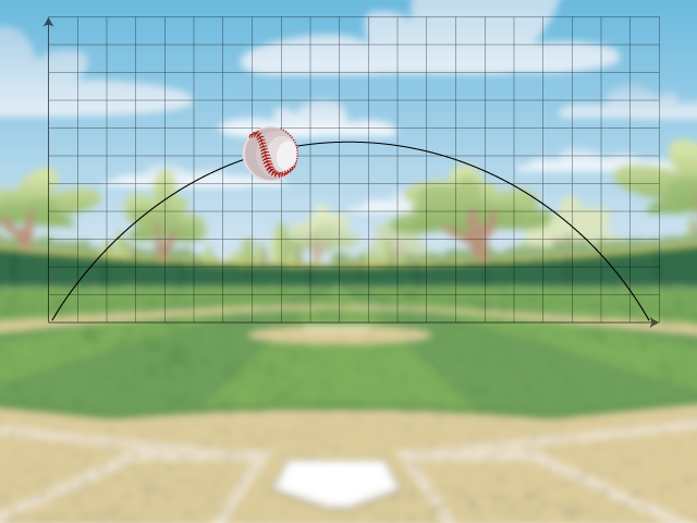
From the illustration you can see that along its parabolic path the baseball moves up and down vertically and across horizontally. Along any part of its path the baseball has a horizontal and vertical component of motion.

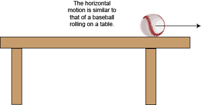
Focusing just on the horizontal motion of the ball, it is actually moving at a constant speed, as if the ball were rolling on a table.

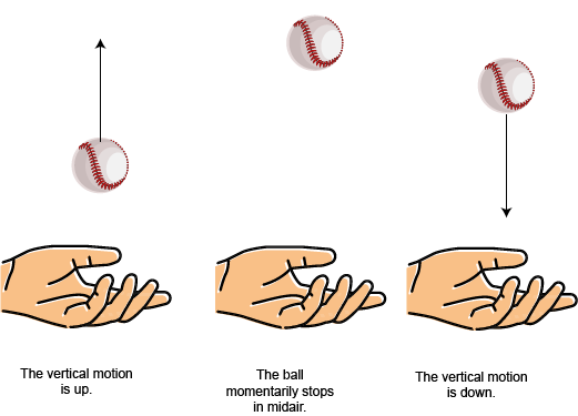
Now focusing just on the vertical motion of the ball, it is similar to the motion of someone tossing a ball up and down. This up-and-down motion is not constant: The ball moves up, stops in midair at some point, and then drops down.

Both the horizontal and vertical components of motion are independent of each other:

• No matter how fast the ball is traveling horizontally, it will have no impact on how it travels vertically.
• No matter how high the ball is thrown, it will have no impact on its horizontal speed.

What both the horizontal and vertical motions are dependent on is the amount of time the ball is in the air. This means that both x and y are functions of the variable t, or time.

There are two functions

Let’s examine each function independently.

Horizontal Motion

We saw earlier that the horizontal motion of the ball is a constant speed. Let’s designate this constant speed with the variable s. To find the horizontal distance traveled for time t, use this equation

This equation shows that x is a function of time, t. Notice that x(t) is a linear function. The slope of the linear function is the horizontal speed of the ball.

Now let’s look at vertical motion.

Vertical Motion

Vertical motion has to take gravity into account:

• On the way up, gravity slows down the ball.
• At its highest point, the ball is momentarily stopped.
• On the way down, gravity speeds up the ball. 

To find the vertical distance traveled for time t, use this equation

In this equation, v is the initial vertical speed that the ball has. That’s the speed that is slowed down and accelerated by gravity.

Parametric Equations

We now have the horizontal and vertical equations of motion:

Each of these equations is a function of the variable t, for time. To graph a parametric equation, think of the ordered pairs that result for different values of t.

Parametric Equations: Example

Let’s look at a specific example. Suppose a baseball player throws a ball with these speed parameters:

Horizontal speed: 50 ft/sec

Vertical speed: 25 ft/sec

The parametric equations become

Let’s create a table of values for different values of t, starting at t = 0.

Notice that after 2 seconds the y value is already negative. What does this mean? Since y represents the height of the ball above the ground, then y can’t be zero. 

You can see that a ball needs a high vertical speed in order for it to travel a longer horizontal distance. You can also increase the horizontal speed. Try this set of parametric equations.

Here is a graph of these coordinates.

Can you see the parabolic shape of the graph?

You can explore different parameters using the Desmos graphing calculator. In the activity below change the values for a and b, which represent the horizontal and vertical speeds, until the ball lands at (0, 450).

 

Set the horizontal and vertical speeds of the ball to have the ball land on coordinates (450, 0).

Summary

 

Parametric equations are a way to express the coordinates of a point in a plane (usually in 2D space) as functions of one or more independent parameters. Instead of describing the position of a point with a single equation relating x and y, parametric equations use separate equations for x and y, each in terms of a parameter, typically denoted as "t" or another letter.

Parametric equations are often used to describe the motion or path of an object over time. They are particularly useful when dealing with complex or curved trajectories. Here's a basic explanation of parametric equations:

1. Parameter: The parameter (usually denoted as "t") is a variable that represents the progress along the path or the passage of time. It is not necessarily restricted to time, but it often represents time in dynamic scenarios.

2. Equations for x and y: You have two separate equations, one for x and one for y, each expressed as a function of the parameter "t." These equations define how the x and y coordinates of a point change as the parameter "t" varies.

   • x = f(t)
   • y = g(t)

3. The Parametric Curve: By varying the parameter "t," you can generate a series of points (x, y) that collectively trace out a curve in the plane. This curve is called the parametric curve.

4. Parameter Domain: The parameter "t" often has a specified domain, which determines the range of values it can take. This domain helps control how much of the curve is plotted.

5. Examples: Parametric equations can be used to describe a wide range of curves, including lines, circles, ellipses, parabolas, and more complex shapes. For example, the parametric equations for a circle with radius "r" centered at the origin are:

   • x = r * cos(t)
   • y = r * sin(t)

   Here, "t" varies from 0 to 2π to trace out the entire circle.

Parametric equations are valuable in various fields, including physics, engineering, computer graphics, and mathematics, as they provide a flexible way to represent complex curves and dynamic processes. They are also used in calculus to calculate things like arc length and the curvature of curves.