What Are Piecewise Functions?

In your work with functions you are accustomed to seeing continuous functions that extend to infinitely on either end. Here are examples of such functions.

But there is another family of functions that you can see in this Venn diagram.

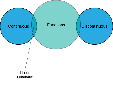
Continuous functions like linear and quadratic are functions that you’re familiar with, but there are discontinuous functions, too. Let’s look at those as we begin to explore piecewise functions.

Functions with Points of Discontinuity

A function is discontinuous if there are certain points in the domain where the behavior of the function changes. There are certain functions that have discontinuous behavior. Let’s look at a simple example:

What happens when x approaches zero? Do you see that this function is undefined at x = 0?

Here is a graph of this function.

As x approaches zero from the left, notice that the function approaches negative infinity. As x approaches zero form the right, the function approaches positive infinity. The function f(x) = 1/x is not defined at x = 0. This is a point of discontinuity.

As a result, the domain of this rational function does not include zero. That means that rational functions are continuous over the domain (which doesn’t include x = 0).

Discontinuous Functions

A function is discontinuous if it shows a break or gap for certain values in its domain.

Notice that although there is a gap in the function, the graph still passes the vertical line test. Now we can look at piecewise functions.

Not all discontinuous functions need to have a noticeable gap. Take a look at the graph of an absolute value function.

While it may look continuous, let’s explore its discontinuity. 

An absolute value function is made up of two linear components that intersect at one point. Let’s look at each linear function separately.

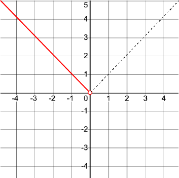
The linear function on the left ends at the origin but doesn’t include that point. The limit as x approaches zero is zero. However f(0) is not defined for this linear function. Now let’s look at the other linear function.

This function does include the origin. (Both functions can’t include the origin without violating the vertical line test.) The limit as x approaches zero is zero, and for this function f(0) is defined.

As a result the absolute value function is discontinuous. The discontinuity is based on the fact that at the point a where the graph changes direction the value of f(a) exists for one graph but not for the other.

Piecewise Functions

Piecewise functions are discontinuous functions made up of functional components. Think of stitching together a function from portions of continuous functions. 

Take a look at this graph.

This function is made up of pieces of three continuous functions: a linear function, a quadratic function, and a linear function. Each of these pieces are strung together to form a discontinuous piecewise function. 

Let’s look at an example.

Example: Step Functions

A step function is a special type of piecewise function that has only a finite number of pieces. In other words, the function is defined differently over a finite number of intervals. Step functions are often used to model real-world phenomena that have a discrete or quantized nature, such as digital signals, voltage levels, and temperature thresholds.

Here is a simple example of a step function:

This function has two pieces:

• For all values of x between 0 and 1, not including those values, the function is equal to 0.
• For all values of x between 1 and 2, including 1, the function is equal to 1.

This is what the graph of this function looks like:

See the stair-step pattern. A more general version is the floor function.

The floor function takes every input value and outputs the lowest integer value. For example floor(1.2) = 1.

There is also the ceiling function, whose graph looks like this.

Step functions can be more complex than the examples above, but they always work in the same way: we determine which piece of the function applies to the input value, and then we evaluate that piece.

Step functions are used in many different areas of mathematics, science, and engineering. For example, they are used to model the behavior of digital circuits, the quantization of audio signals, and the discretization of time in computer simulations.

Here are some examples of step functions in the real world:

• A thermostat that turns on a heater when the temperature drops below a certain threshold.
• A digital clock that displays the current time in hours and minutes.
• A traffic light that turns red when a pedestrian button is pressed.
• A video game that displays different images on the screen depending on the player's actions.

Step functions are a versatile and powerful tool for modeling real-world phenomena. They are also relatively easy to understand and implement, which makes them a popular choice for many applications.

Summary

A piecewise function is a function that is defined differently over different intervals. This means that the function has different equations depending on the value of the input variable. Piecewise functions are often used to model real-world phenomena that are complex or have multiple different states.

Here is a simple example of a piecewise function:

This function has three different pieces:

• For all values of x less than 0, the function is equal to x + 1.
• For all values of x between 0 and 3, the function is equal to 2x - 3.
• For all values of x greater than or equal to 3, the function is equal to x^2 + 2.

To evaluate this function for a given input value, we simply need to determine which piece of the function applies to that value. For example, if we want to evaluate f(x) for x = -2, we see that x < 0, so we use the first equation:

If we want to evaluate f(x) for x = 2, we see that 0 ≤ x < 3, so we use the second equation:

And if we want to evaluate f(x) for x = 4, we see that x ≥ 3, so we use the third equation:

Here is the graph of the piecewise function.

Piecewise functions can be more complex than the example above, but they always work in the same way: we determine which piece of the function applies to the input value, and then we evaluate that piece.

Piecewise functions are used in many different areas of mathematics, science, and engineering. For example, they are used to model the behavior of electrical circuits, the motion of projectiles, and the spread of diseases.