Lesson Plan: Linear Functions and Applications 

Lesson Summary

In this lesson, students will deepen their understanding of linear functions by exploring their real-world applications. They will learn to represent linear functions using equations, tables, and graphs, and apply these representations to solve practical problems. The lesson emphasizes identifying the domain and range of linear functions and interpreting the significance of slope and y-intercept in various contexts. Through interactive activities and discussions, students will recognize how linear functions model relationships in everyday life, such as calculating costs, predicting distances, and analyzing patterns.

Lesson Objectives

• Understand the concept of linear functions
• Identify the domain and range of a linear function
• Represent linear functions using equations, tables, and graphs
• Apply linear functions to solve real-world problems

Common Core Standards

• 8.F.A.1: Understand that a function is a rule that assigns to each input exactly one output.
• 8.F.A.3: Interpret the equation y = mx + b as defining a linear function, whose graph is a straight line.

Prerequisite Skills

• Understanding of linear equations
• Graphing linear equations
• Interpreting slope and y-intercept

Key Vocabulary

• Function – A relationship that assigns exactly one output value for each input value. Functions can be represented in equations, tables, graphs, or verbal descriptions.
• Linear Function – A function whose graph is a straight line. It can be expressed in the form $y = mx + b$, where $m$ is the slope and $b$ is the y-intercept.
• Domain – The set of all possible input values ($x$) for which a function is defined.
• Range – The set of all possible output values ($y$) that a function can produce.
• Input – The independent variable in a function, commonly represented by $x$.
• Output – The dependent variable in a function, commonly represented by $y$.
• Slope ($m$) – A measure of the steepness of a line, calculated as: $$m = \frac{\Delta y}{\Delta x}$$
• Y-Intercept ($b$) – The point where the graph of a function crosses the y-axis. In $y = mx + b$, $b$ is the y-intercept.
• Linear Model – A linear equation that represents a real-world situation, describing relationships with a constant rate of change.
• Constant Rate of Change – The unchanging rate at which one quantity changes relative to another in a linear relationship, represented by the slope.
• Independent Variable – The variable that represents the input or cause in a function. In $y = f(x)$, $x$ is the independent variable.
• Dependent Variable – The variable that represents the output or effect and depends on the input. In $y = f(x)$, $y$ is the dependent variable.

 Multimedia Resources

• Math definitions of terms related to linear equations and functions: https://www.media4math.com/Definitions--LinearFunctions
• Video definitions on the topic of linear equations and functions: https://www.media4math.com/MathVideoCollection--LinearFunctionsDefinitions

Warm Up Activities

Choose from one or more of the following activities

Activity1: Identifying Linear Functions from Tables

Students will analyze data tables and determine whether the relationship is linear by checking for a constant rate of change.

Instructions:

• Provide students with the following data table and ask them to determine if the relationship is linear.
• Have students calculate the change in $y$ for each change in $x$.
• If the rate of change remains constant, then the function is linear.

Data Table:

Solution: The rate of change is calculated as:

$$m = \frac{y_2 - y_1}{x_2 - x_1} = \frac{6 - 3}{2 - 1} = 3$$

Since the rate of change is constant, the data represents a linear function with an equation $y = 3x$.

Activity 2: Matching Graphs to Equations

Students will match given linear equations to their corresponding graphs.

Instructions:

• Provide students with a set of graphs and ask them to match each to the correct equation.
• Encourage them to analyze slope and y-intercept for quick identification.

Graph Specifications:

The following equations should be graphed for students:

• Graph 1: $y = 2x + 1$
  • Slope: $2$ (line rises 2 units for every 1 unit to the right)
  • Y-Intercept: $(0,1)$
• Graph 2: $y = -\frac{1}{2}x + 3$
  • Slope: $-\frac{1}{2}$ (line falls 1 unit for every 2 units to the right)
  • Y-Intercept: $(0,3)$
• Graph 3: $y = 4x$
  • Slope: $4$ (steep increasing line passing through origin)
  • Y-Intercept: $(0,0)$
• Graph 4: $y = -x + 5$
  • Slope: $-1$ (line falls at a 45-degree angle)
  • Y-Intercept: $(0,5)$

Graph 1	Graph 2	Graph 3	Graph 4

Discussion Questions:

• How does the slope affect the direction of the line?
• What happens when the y-intercept changes?
• How can you quickly determine the equation of a line from a graph?

Activity 3: Desmos Activity: Graphing Linear Equations in Standard Form

Students will use Desmos to explore the graphs of linear equations in standard form ($Ax + By = C$).

Activity Steps:

• Have students enter equations like $2x + 3y = 6$ into Desmos.
• Observe how changing $A$, $B$, and $C$ affects the graph.
• Identify x- and y-intercepts by setting $x = 0$ and $y = 0$.

Discuss findings and compare how equations in standard form differ from slope-intercept form.

Activity 4: Review of Slope

Students will review the concept of slope by working through examples with the slope formula:

$$m = \frac{y_2 - y_1}{x_2 - x_1}$$

Activity Steps:

• Provide students with two points, such as (1, 2) and (4, 8).
• Have them apply the formula to calculate the slope:
• $$m = \frac{8 - 2}{4 - 1} = \frac{6}{3} = 2$$
• Discuss what positive, negative, zero, and undefined slopes look like on a graph.

Activity 5: Graphing Ordered Pairs

Ask students to identify patterns in a set of ordered pairs, such as 

(1, 3)

(2, 5)

(3, 7)

(4, 9)

Guide them to recognize that the y-values increase by 2 for each increase of 1 in the x-values, representing a linear relationship.

Use this Desmos activity to graph these ordered pairs. Ask students to predict the next two sets of ordered pairs. Have them make a conclusion about the graph.

https://www.desmos.com/calculator/nqqzl2dkc6

Teach

Definitions

Define a function as a rule that assigns to each input exactly one output. Use the following slide show:

https://www.media4math.com/library/slideshow/function-representations

 The slide show introduces linear functions as a specific type of function where the output (y-value) changes at a constant rate as the input (x-value) changes.

• Explain the equation y = mx + b, where m represents the slope (rate of change) and b represents the y-intercept.

Use this slide show to go over the key ideas around graphs of linear functions:
https://www.media4math.com/library/slideshow/graphs-linear-functions

Demonstrate how to represent linear functions using equations, tables, and graphs. Use this slide show:

https://www.media4math.com/library/slideshow/multiple-representations-linear-equations

Discuss the domain and range of linear functions, emphasizing that the domain is the set of all possible input values, and the range is the set of all possible output values. Use this slide show of definitions:

https://www.media4math.com/library/slideshow/function-definitions

Examples 

Provide examples and non-examples of linear functions to reinforce understanding. Use this slide show to demonstrate non-linear function graphs:

https://www.media4math.com/library/slideshow/non-linear-function-graphs

Use this slide show to look at examples of finding the domain and range of a function:

https://www.media4math.com/library/slideshow/domain-and-range-functions-linear

Applications

The following are slide shows that go into detailed analysis of applications of linear functions. Choose one of these slide shows to show an application of linear functions:

Review

Summary of the Lesson

In this lesson, students explored linear functions and their applications in real-world contexts. They learned how to represent linear functions using equations, tables, and graphs, and analyzed key characteristics such as slope, y-intercept, domain, and range.

Students also practiced identifying linear relationships in different representations and applied their knowledge to model real-world problems such as cost analysis, motion over time, and savings growth.

The lesson emphasized how linear functions describe relationships with a constant rate of change and how these functions can be used to make predictions.

Key Vocabulary

• Function – A relationship where each input value has exactly one output value. Functions can be represented using equations, tables, graphs, or verbal descriptions.
• Linear Function – A function whose graph is a straight line. It has the standard form $y = mx + b$, where $m$ represents the slope and $b$ is the y-intercept.
• Domain – The set of all possible input values ($x$) for which a function is defined.
• Range – The set of all possible output values ($y$) that a function can produce.
• Input – The independent variable in a function, commonly represented by $x$.
• Output – The dependent variable in a function, commonly represented by $y$.
• Slope ($m$) – The measure of steepness of a line, calculated as: $$m = \frac{\Delta y}{\Delta x}$$
• Y-Intercept ($b$) – The point where the graph of a function crosses the y-axis. In $y = mx + b$, $b$ is the y-intercept.
• Linear Model – A linear equation that represents a real-world situation, describing relationships with a constant rate of change.
• Constant Rate of Change – The unchanging rate at which one quantity changes relative to another in a linear relationship, represented by the slope.
• Independent Variable – The variable that represents the input or cause in a function. In $y = f(x)$, $x$ is the independent variable.
• Dependent Variable – The variable that represents the output or effect and depends on the input. In $y = f(x)$, $y$ is the dependent variable.
• X-Intercept – The point where a line crosses the x-axis ($y = 0$).
• Proportional Relationship – A special case of a linear function where the line passes through the origin ($y = mx$), meaning there is no y-intercept ($b = 0$).

Discussion

• Engage students in a discussion by asking them to identify real-world situations that can be modeled using linear functions.
• Provide a few examples, such as calculating the cost of renting a car based on a daily rate and a one-time fee, or determining the distance traveled based on a constant speed.
• Use one of the applications of linear functions shown in the previous section to review another application.
• Encourage students to share their own examples and explain how they would represent the situation using a linear function.

Quiz

Answer the following questions.

1. Which of the following is true about a function?
   a) An input value can have more than one output value.
   b) An input value has one output value.
   c) Two input values can have the same output value.
   d) An input value cannot be zero.
2. Define a linear function.
3. What does the slope (m) represent in the equation y = mx + b?
4. If a linear function has a slope of 3 and a y-intercept of 2, what is the equation of the function?
5. Given the ordered pairs (0, 2), (1, 4), (2, 6), (3, 8), identify the linear function represented by these points.
6. What is the domain of the linear function y = 2x - 3?
7. What is the range of the linear function y = -x + 5?
8. Represent the linear function y = 4x - 1 using a table of values.

9. Graph the linear function y = -2x + 3.
    

   

10. A car rental company charges \$25 per day plus a one-time fee of \$15. Write a linear function to represent the total cost of renting the car for x days.

Answer Key

1. b) and c)
2. A linear function is of the form y = mx + b, whose graph is a line.
3. The slope (m) represents the rate of change or the constant rate at which the output changes for each unit change in the input.
4. y = 3x + 2
5. y = 2x + 2
6. The domain is the set of all real numbers.
7. The range is the set of all real numbers.
8. x | y
   0 | -1
   1 | 3
   2 | 7
   3 | 11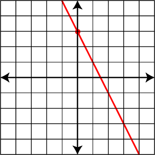
9. 
10. Total cost = 25x + 15

Purchase the lesson plan bundle. Click here.