Lesson Plan: Understanding Direct Variation and Its Connection to Proportional Relationships

Lesson Summary

In this lesson, students will explore direct variation, a specific type of proportional relationship where one variable is a constant multiple of another. They will learn how to identify direct variation in tables, equations, and graphs, and how to determine the constant of variation. This lesson will strengthen their understanding of proportional relationships and linear functions, preparing them for more advanced algebraic concepts.

Students will practice:

• Identifying direct variation relationships in equations, tables, and graphs.
• Understanding the equation of a direct variation: $y = kx$, where $k$ is the constant of variation.
• Determining the constant of variation from different representations.
• Graphing direct variation functions and recognizing their key characteristics.
• Applying direct variation to real-world problems, such as speed-time and force-mass relationships.

By the end of this lesson, students will be able to analyze and interpret direct variation relationships and understand their connection to linear equations.

Lesson Objectives

• Understand the concept of direct variation
• Recognize direct variation as a special case of linear relationships where y = kx (k is the constant of variation)
• Interpret the meaning of the constant of variation in real-world contexts
• Graph direct variation equations
• Compare different direct variation relationships
• Derive direct variation relationships from real-world data sets

Common Core Standards

• CCSS.MATH.CONTENT.8.EE.B.5
  Graph proportional relationships, interpreting the unit rate as the slope of the graph. Compare two different proportional relationships represented in different ways.
• CCSS.MATH.CONTENT.8.F.B.4
  Construct a function to model a linear relationship between two quantities. Determine the rate of change and initial value of the function from a description of a relationship or from two (x, y) values, including reading these from a table or from a graph. Interpret the rate of change and initial value of a linear function in terms of the situation it models, and in terms of its graph or a table of values.

Prerequisite Skills

• Graphing on a coordinate plane
• Understanding of proportional relationships
• Basic knowledge of linear equations

Key Vocabulary

• Direct Variation: A proportional relationship between two variables where one variable is a constant multiple of the other.
• Constant of Variation: The constant $k$ in the equation $y = kx$, representing the ratio between $y$ and $x$.
  • Multimedia Resource: https://www.media4math.com/library/43411/asset-preview
• Proportional Relationship: A relationship where the ratio between two variables remains constant.
  • Multimedia Resource: https://www.media4math.com/library/43387/asset-preview
• Linear Equation: An equation that forms a straight line when graphed; in direct variation, this is represented as $y = kx$.
• Origin: The point (0,0) on a coordinate plane where a direct variation graph always passes through.
• Slope: The rate of change between two variables in a linear function; in direct variation, the slope is the constant of variation.
  • Multimedia Resource: https://www.media4math.com/library/74617/asset-preview
• Table of Values: A table showing corresponding values for $x$ and $y$ in a direct variation relationship.
• Graph of a Direct Variation: A straight line passing through the origin, representing a direct variation relationship.

Multimedia Resources

• A collection of definitions on the topic of ratios, proportions, and percents: https://www.media4math.com/Definitions--RatiosProportionsPercents
• A student tutorial slide show on definitions on the topic of ratios, proportions, and percents: https://www.media4math.com/library/slideshow/student-tutorial-ratios-proportions-and-percents-definitions
• A slide show of definitions related to the topic of Direction Variations: https://www.media4math.com/library/slideshow/direct-variation-definitions

Warm Up Activities

Choose from one or more activities.

Activity 1: Review of Proportional Relationships

Start the lesson by reviewing proportional relationships and their key characteristics.

Example: A car travels 200 miles in 4 hours. Is this a proportional relationship?

Solution:

• Find the unit rate: $$\frac{200}{4} = 50 \text{ miles per hour}$$
• Since the rate remains constant, the relationship is proportional.

Activity 2: Review of Constant of Proportionality

Remind students that the constant of proportionality ($k$) represents the constant ratio in a proportional relationship.

Example: A bakery sells 3 cupcakes for $6. What is the constant of proportionality?

Solution:

• Use the formula for the constant of proportionality: $$k = \frac{\text{Output (y)}}{\text{Input (x)}}$$
• Substituting the given values: $$k = \frac{6}{3} = 2$$

Thus, the constant of proportionality is 2, meaning each cupcake costs $2.

Activity 3: Review of Slope as Rate of Change

Since direct variation graphs form a straight line, it's important to review slope as the rate of change between two variables.

Formula for Slope:

$$m = \frac{y_2 - y_1}{x_2 - x_1}$$

Example: Given the points (2,4) and (5,10), find the slope.

Solution:

• Apply the slope formula: $$m = \frac{10 - 4}{5 - 2} = \frac{6}{3} = 2$$

Thus, the slope of the line is 2, meaning the value of $y$ increases by 2 for every 1 unit increase in $x$.

Activity 4: Application of Proportional Relationships

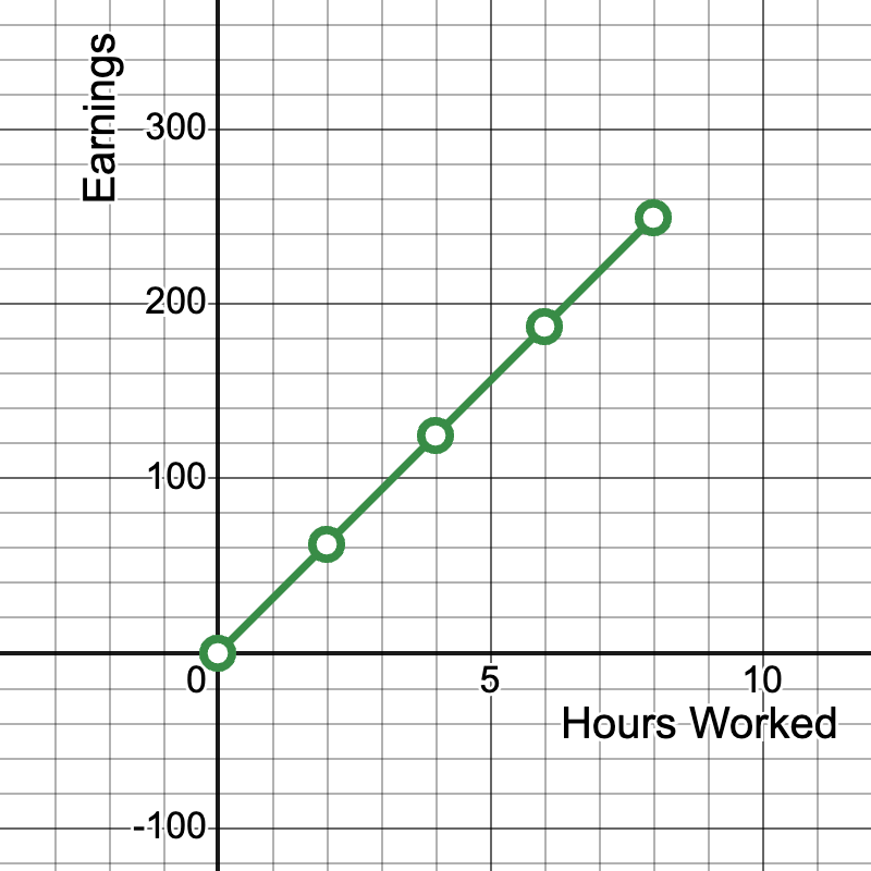
Students are presented with the following real-world data set showing the relationship between hours worked and total earnings based on the average hourly wage in the United States (data from Bureau of Labor Statistics, 2021):

Students are asked to:

1. Plot these points on a coordinate plane
2. Determine if they form a straight line through the origin
3. Calculate the average hourly wage (slope of the line)
4. Write the direct variation equation for this relationship

Here is the graph of the data, with a line connecting the data points:

Here is a Desmos activity you can use:

https://www.desmos.com/calculator/hsxpiioouh

Teach

Understanding Direct Variation

Direct variation is a relationship between two variables where one variable is always a constant multiple of the other. This means that as one variable increases, the other increases proportionally.

Equation of Direct Variation:

$$y = kx$$

where:

• $y$ is the dependent variable.
• $x$ is the independent variable.
• $k$ is the constant of variation (or proportionality).

Example: If $y$ varies directly with $x$ and $k = 3$, write the equation.

Solution:

• Since direct variation follows $y = kx$, substitute $k = 3$: $$y = 3x$$

Identifying Direct Variation in Tables

A table represents direct variation if the ratio $\frac{y}{x}$ remains constant for all values.

Example: Does the following table represent a direct variation?

Solution:

• Calculate $\frac{y}{x}$ for each row: $$\frac{6}{2} = 3, \quad \frac{12}{4} = 3, \quad \frac{18}{6} = 3$$
• Since the ratio remains constant, the relationship represents a direct variation with $k = 3$.

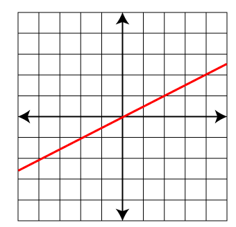
Graphing Direct Variation

Direct variation graphs are straight lines that pass through the origin (0,0) and have a slope equal to the constant of variation.

Example: Graph the direct variation equation $y = 4x$.

Steps:

1. Create a table of values:

2. Plot the points on a coordinate plane.
3. Draw a straight line through the points, ensuring it passes through the origin.

Since the graph is a straight line through the origin, it confirms a direct variation.

Determining the Constant of Variation

The constant of variation ($k$) can be found using the formula:

$$k = \frac{y}{x}$$

Example: If $y = 15$ when $x = 5$, find the constant of variation.

Solution:

• Apply the formula: $$k = \frac{15}{5} = 3$$

Thus, the constant of variation is 3, meaning the equation is $y = 3x$.

Real-World Applications of Direct Variation

Direct variation is used in many real-world scenarios where two quantities increase or decrease proportionally.

Example 1: Speed and Time

A car travels at a constant speed of 60 miles per hour. Write the direct variation equation for the relationship between distance and time.

Solution:

• Let $y$ represent the distance traveled and $x$ represent time in hours.
• Since the car travels 60 miles per hour, $k = 60$, so the equation is: $$y = 60x$$

Example 2: Earnings and Hours Worked

A worker earns $12 per hour. How much will they earn in 5 hours?

Solution:

• Since earnings vary directly with hours worked, the equation is: $$y = 12x$$
• Substituting $x = 5$: $$y = 12 \times 5 = 60$$

Thus, the worker will earn $60 in 5 hours.

Definitions

• Direct variation: A relationship between two variables where one is a constant multiple of the other, expressed as y = kx.
• Constant of variation: The constant k in the direct variation equation y = kx, representing the ratio of y to x.
• Proportional relationship: A relationship where the ratio of two quantities remains constant as the quantities change.
• Linear function: A function whose graph is a straight line, often written in the form y = mx + b.
• Slope-intercept form: The equation of a line written as y = mx + b, where m is the slope and b is the y-intercept.

Use this slide show to review these and other definitions:

https://www.media4math.com/library/slideshow/direct-variation-definitions

Introduce direct variations with this video:

https://www.media4math.com/library/44915/asset-preview

Explain the concept of direct variation (y = kx, where k is the constant of variation), demonstrate how direct variation is a special case of linear relationships where the y-intercept is zero, show how to graph direct variation equations, and explain how the constant of variation relates to the slope and unit rate in proportional relationships.

Example 1: Circumference and Diameter of a Circle

Use this slide show with this example:

https://www.media4math.com/library/slideshow/applications-direct-variations-circles

The circumference (C) of a circle varies directly with its diameter (D).

• Write the direct variation equation.
• Calculate the circumference of a circle with a diameter of 10 cm.
• Interpret the constant of variation.

Solution:

• Equation: C = πD, where C is the circumference and D is the diameter
• Circumference: C = π(10) ≈ 31.42 cm
• The constant of variation (π) represents the ratio of circumference to diameter for all circles

This Desmos activity can be used to support this activity:

https://www.desmos.com/calculator/sthkxtueqj

Example 2: Hooke's Law

Use this slide show to accompany this example:

https://www.media4math.com/library/slideshow/application-linear-functions-hookes-law

Hooke's Law states that the force (F) needed to extend or compress a spring by some distance (x) varies directly with that distance.

• Write the direct variation equation for Hooke's Law.
• If a force of 50 N extends a spring by 0.25 m, what is the spring constant?
• Calculate the force needed to extend the same spring by 0.4 m.

Solution:

• Equation: F = kx, where F is the force, x is the displacement, and k is the spring constant
• Spring constant: k = F/x = 50/0.25 = 200 N/m
• Force for 0.4 m extension: F = 200(0.4) = 80 N

Example 3: Currency Exchange

Use this slide show to accompany this example:

https://www.media4math.com/library/slideshow/applications-proportions-exchange-rates

The exchange rate between US dollars and euros is 1 USD = 0.85 EUR.

• Write the direct variation equation.
• Calculate how many euros 120 USD would exchange for.
• Interpret the constant of variation.

Solution:

• Equation: e = 0.85d, where e is euros and d is US dollars
• Euros: e = 0.85(120) = 102 EUR
• The constant of variation (0.85) represents the exchange rate

Example 4: AI-Enabled Smartphone Revenue

A tech company has collected data on the number of AI-enabled smartphones sold and the corresponding revenue:

• Plot these points on a coordinate plane.
• Determine if they form a straight line through the origin.
• Calculate the revenue per unit sold (slope of the line).
• Write the direct variation equation for this relationship.
• Use the equation to predict the revenue for 500 units sold.

Solution:

• The points form a straight line through the origin when plotted.
   

   

  

   

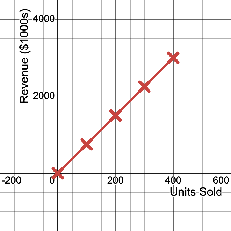
• Slope (revenue per unit) = 3000/400 = 7.5
• Direct variation equation: y = 7.5x, where y is revenue in $1000s and x is units sold
• For 500 units: y = 7.5(500) = 3750
• The company can expect $3,750,000 in revenue from selling 500 units.

Here is a Desmos activity you can use:

https://www.desmos.com/calculator/gsao4ev7lw 

Review

Lesson Summary

In this lesson, students explored direct variation as a special type of proportional relationship where one variable is a constant multiple of another. They learned that direct variation is represented by the equation $y = kx$, where $k$ is the constant of variation. Through equations, tables, and graphs, students identified direct variation relationships and analyzed their characteristics.

Key takeaways from this lesson include:

• Understanding Direct Variation: A direct variation relationship follows the equation $y = kx$, meaning that as $x$ increases or decreases, $y$ changes proportionally.
• Identifying Direct Variation in Tables: If the ratio $\frac{y}{x}$ remains constant for all values in a table, the relationship represents direct variation.
• Graphing Direct Variation: A direct variation graph is always a straight line that passes through the origin (0,0) and has a slope equal to the constant of variation ($k$).
• Determining the Constant of Variation: The constant $k$ can be found using the formula: $$k = \frac{y}{x}$$ for any point in a direct variation relationship.
• Real-World Applications: Direct variation is commonly seen in real-world scenarios, such as speed and time, wages and hours worked, and force and mass relationships.

Example 1 (Art): Mural Paint Calculation

A mural artist has found that the amount of paint used is directly proportional to the wall area. For every 3 square feet of wall, 1 ounce of paint is used.

• Write the direct variation equation.
• Calculate the amount of paint needed for a 150 square foot mural.
• If the artist has 60 ounces of paint, what size mural can they complete?

Solution:

• Equation: P = (1/3)A, where P is the amount of paint in ounces and A is the wall area in square feet
• Paint needed for 150 sq ft: P = (1/3)(150) = 50 ounces
• Mural size with 60 ounces: A = 3P = 3(60) = 180 square feet

Example 2 (Technology): Data Transfer Rate

In a fiber optic network, the amount of data transferred is directly proportional to the time of transfer. The transfer rate is 100 megabits per second.

• Write the direct variation equation.
• How much data can be transferred in 5 minutes?

Solution:

• Equation: D = 100t, where D is the amount of data in megabits and t is the time in seconds
• Data transferred in 5 minutes: D = 100(5 * 60) = 30,000 megabits = 30 gigabits

Example 3 (Nature): Photosynthesis and Light Intensity

The rate of photosynthesis in a plant is directly proportional to light intensity (within a certain range). If the rate of photosynthesis is 2 μmol CO₂/m²/s at a light intensity of 100 μmol photons/m²/s:

• Write the direct variation equation.
• Predict the photosynthesis rate at a light intensity of 250 μmol photons/m²/s.

Solution:

• Equation: R = 0.02I, where R is the rate of photosynthesis in μmol CO₂/m²/s and I is the light intensity in μmol photons/m²/s
• Photosynthesis rate at 250 μmol photons/m²/s: R = 0.02(250) = 5 μmol CO₂/m²/s

Quiz

Answer the following questions.

1. Write the direct variation equation for y varying directly as x with a constant of variation of 3.
   
    
2. What is the constant of variation in the equation y = 2.5x?
   
    
3. Graph the direct variation equation y = 0.5x.
   
   
    
4. If y varies directly as x, and y = 12 when x = 4, what is the constant of variation?
   
    
5. In a direct variation, if x increases by 2, y increases by 6. What is the constant of variation?
   
    
6. Write an equation for a direct variation that passes through the point (2, 10).
   
    
7. How does the graph of y = 3x compare to y = 2x?
   
    
8. In the equation y = 40x, where y is total cost and x is the number of items, what does 40 represent?
   
    
9. If distance varies directly as time, and a car travels 240 miles in 4 hours, write the direct variation equation.
   
    
10. Explain why all direct variation equations represent proportional relationships.
    
     

Answer Key

1. y = 3x
2. 2.5
3. 
4. 3
5. 3
6. y = 5x
7. y = 3x has a steeper slope
8. The cost per item
9. d = 60t, where d is distance in miles and t is time in hours
10. In direct variations, y = kx, which always passes through (0,0) and has a constant ratio y/x = k, meeting the definition of a proportional relationship.

Purchase the lesson plan bundle. Click here.