
Illustrative Math Alignment: Grade 8 Unit 6
Associations in Data
Lesson 11: Gone In 30 Seconds
Use the following Media4Math resources with this Illustrative Math lesson.
| Thumbnail Image | Title | Body | Curriculum Topic |
|---|---|---|---|
|
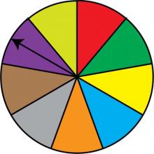
Math Clip Art: Spinner, 9 Sections--Result 8 | Math Clip Art: Spinner, 9 Sections--Result 8TopicProbability and Statistics DescriptionThis image showcases a spinner divided into nine equal sections colored red, green, dark yellow, light blue, orange, grey, brown, purple, and light yellow. The spinner's arrow points to the purple section, illustrating another possible outcome in this probability model. In the context of Probability and Statistics, this spinner represents a probability experiment with nine equally likely outcomes. It visually demonstrates the concepts of sample space and individual events within that space, each with a 1/9 probability of occurrence. |
Probability |
|
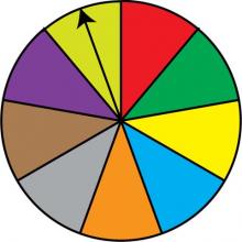
Math Clip Art: Spinner, 9 Sections--Result 9 | Math Clip Art: Spinner, 9 Sections--Result 9TopicProbability and Statistics DescriptionThis image displays a spinner divided into nine equal sections colored red, green, dark yellow, light blue, orange, grey, brown, purple, and light yellow. The spinner's arrow points to the light yellow section, showcasing the final possible outcome in this probability model. In the field of Probability and Statistics, this spinner exemplifies a uniform probability distribution with nine equally likely outcomes. Each spin has a 1/9 probability of landing on any given color, illustrating the concept of equiprobable events in a more complex scenario. |
Probability |
|
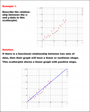
Math Example--Charts, Graphs, and Plots--Analyzing Scatterplots: Example 1 | Math Example--Charts, Graphs, and Plots-- Analyzing Scatterplots: Example 1
In this set of math examples, analyze the behavior of different scatterplots. This includes linear and quadratic models. |
Data Analysis |
|
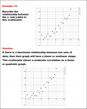
Math Example--Charts, Graphs, and Plots--Analyzing Scatterplots: Example 10 | Math Example--Charts, Graphs, and Plots-- Analyzing Scatterplots: Example 10
In this set of math examples, analyze the behavior of different scatterplots. This includes linear and quadratic models. |
Data Analysis |
|
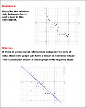
Math Example--Charts, Graphs, and Plots--Analyzing Scatterplots: Example 2 | Math Example--Charts, Graphs, and Plots-- Analyzing Scatterplots: Example 2
In this set of math examples, analyze the behavior of different scatterplots. This includes linear and quadratic models. |
Data Analysis |
|
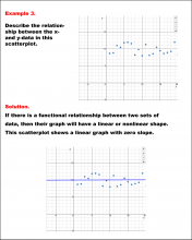
Math Example--Charts, Graphs, and Plots--Analyzing Scatterplots: Example 3 | Math Example--Charts, Graphs, and Plots-- Analyzing Scatterplots: Example 3
In this set of math examples, analyze the behavior of different scatterplots. This includes linear and quadratic models. |
Data Analysis |
|
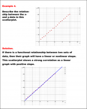
Math Example--Charts, Graphs, and Plots--Analyzing Scatterplots: Example 4 | Math Example--Charts, Graphs, and Plots-- Analyzing Scatterplots: Example 4
In this set of math examples, analyze the behavior of different scatterplots. This includes linear and quadratic models. |
Data Analysis |
|
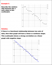
Math Example--Charts, Graphs, and Plots--Analyzing Scatterplots: Example 5 | Math Example--Charts, Graphs, and Plots-- Analyzing Scatterplots: Example 5
In this set of math examples, analyze the behavior of different scatterplots. This includes linear and quadratic models. |
Data Analysis |
|
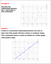
Math Example--Charts, Graphs, and Plots--Analyzing Scatterplots: Example 6 | Math Example--Charts, Graphs, and Plots-- Analyzing Scatterplots: Example 6
In this set of math examples, analyze the behavior of different scatterplots. This includes linear and quadratic models. |
Data Analysis |
|
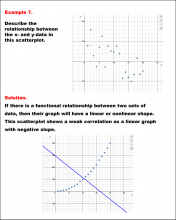
Math Example--Charts, Graphs, and Plots--Analyzing Scatterplots: Example 7 | Math Example--Charts, Graphs, and Plots-- Analyzing Scatterplots: Example 7
In this set of math examples, analyze the behavior of different scatterplots. This includes linear and quadratic models. |
Data Analysis |
|
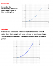
Math Example--Charts, Graphs, and Plots--Analyzing Scatterplots: Example 8 | Math Example--Charts, Graphs, and Plots-- Analyzing Scatterplots: Example 8
In this set of math examples, analyze the behavior of different scatterplots. This includes linear and quadratic models. |
Data Analysis |
|
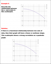
Math Example--Charts, Graphs, and Plots--Analyzing Scatterplots: Example 9 | Math Example--Charts, Graphs, and Plots-- Analyzing Scatterplots: Example 9
In this set of math examples, analyze the behavior of different scatterplots. This includes linear and quadratic models. |
Data Analysis |
|
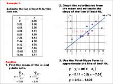
Math Example--Charts, Graphs, and Plots--Estimating the Line of Best Fit: Example 1 | Math Example--Charts, Graphs, and Plots-- Estimating the Line of Best Fit: Example 1
In this set of math examples, analyze the behavior of different scatterplots. This includes linear and quadratic models. |
Slope-Intercept Form and Data Analysis |
|
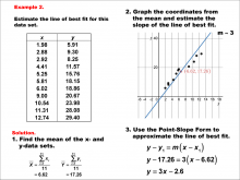
Math Example--Charts, Graphs, and Plots--Estimating the Line of Best Fit: Example 2 | Math Example--Charts, Graphs, and Plots-- Estimating the Line of Best Fit: Example 2
In this set of math examples, analyze the behavior of different scatterplots. This includes linear and quadratic models. |
Point-Slope Form, Slope-Intercept Form and Data Analysis |
|
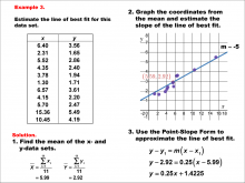
Math Example--Charts, Graphs, and Plots--Estimating the Line of Best Fit: Example 3 | Math Example--Charts, Graphs, and Plots-- Estimating the Line of Best Fit: Example 3
In this set of math examples, analyze the behavior of different scatterplots. This includes linear and quadratic models. |
Point-Slope Form, Slope-Intercept Form and Data Analysis |
|
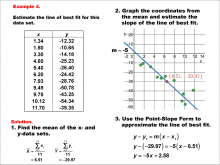
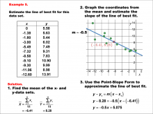
Math Example--Charts, Graphs, and Plots--Estimating the Line of Best Fit: Example 4 | Math Example--Charts, Graphs, and Plots-- Estimating the Line of Best Fit: Example 4
In this set of math examples, analyze the behavior of different scatterplots. This includes linear and quadratic models. |
Point-Slope Form, Slope-Intercept Form and Data Analysis |
|
Math Example--Charts, Graphs, and Plots--Estimating the Line of Best Fit: Example 5 | Math Example--Charts, Graphs, and Plots-- Estimating the Line of Best Fit: Example 5
In this set of math examples, analyze the behavior of different scatterplots. This includes linear and quadratic models. |
Point-Slope Form, Slope-Intercept Form and Data Analysis |

|
Math Example--Charts, Graphs, and Plots--Reading and Interpreting Scaled Graphs--Example 1 | Math Example--Charts, Graphs, and Plots-- Reading and Interpreting Scaled Graphs--Example 1
In this set of math examples, analyze the behavior of different scatterplots. This includes linear and quadratic models. |
Subtraction Facts to 100 and Data Analysis |
|
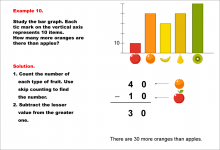
Math Example--Charts, Graphs, and Plots--Reading and Interpreting Scaled Graphs--Example 10 | Math Example--Charts, Graphs, and Plots-- Reading and Interpreting Scaled Graphs--Example 10
In this set of math examples, analyze the behavior of different scatterplots. This includes linear and quadratic models. |
Subtraction Facts to 100 and Data Analysis |
|
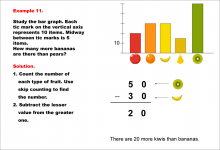
Math Example--Charts, Graphs, and Plots--Reading and Interpreting Scaled Graphs--Example 11 | Math Example--Charts, Graphs, and Plots-- Reading and Interpreting Scaled Graphs--Example 11
In this set of math examples, analyze the behavior of different scatterplots. This includes linear and quadratic models. |
Subtraction Facts to 100 and Data Analysis |
|
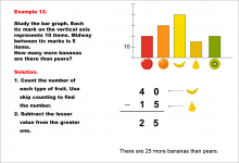
Math Example--Charts, Graphs, and Plots--Reading and Interpreting Scaled Graphs--Example 12 | Math Example--Charts, Graphs, and Plots-- Reading and Interpreting Scaled Graphs--Example 12
In this set of math examples, analyze the behavior of different scatterplots. This includes linear and quadratic models. |
Subtraction Facts to 100 and Data Analysis |
|
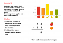
Math Example--Charts, Graphs, and Plots--Reading and Interpreting Scaled Graphs--Example 13 | Math Example--Charts, Graphs, and Plots-- Reading and Interpreting Scaled Graphs--Example 13
In this set of math examples, analyze the behavior of different scatterplots. This includes linear and quadratic models. |
Subtraction Facts to 100 and Data Analysis |
|
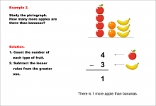
Math Example--Charts, Graphs, and Plots--Reading and Interpreting Scaled Graphs--Example 2 | Math Example--Charts, Graphs, and Plots-- Reading and Interpreting Scaled Graphs--Example 2
In this set of math examples, analyze the behavior of different scatterplots. This includes linear and quadratic models. |
Subtraction Facts to 100 and Data Analysis |
|
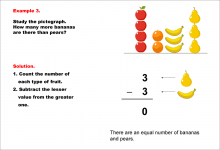
Math Example--Charts, Graphs, and Plots--Reading and Interpreting Scaled Graphs--Example 3 | Math Example--Charts, Graphs, and Plots-- Reading and Interpreting Scaled Graphs--Example 3
In this set of math examples, analyze the behavior of different scatterplots. This includes linear and quadratic models. |
Subtraction Facts to 100 and Data Analysis |
|
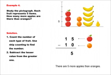
Math Example--Charts, Graphs, and Plots--Reading and Interpreting Scaled Graphs--Example 4 | Math Example--Charts, Graphs, and Plots-- Reading and Interpreting Scaled Graphs--Example 4
In this set of math examples, analyze the behavior of different scatterplots. This includes linear and quadratic models. |
Subtraction Facts to 100 and Data Analysis |
|
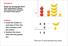
Math Example--Charts, Graphs, and Plots--Reading and Interpreting Scaled Graphs--Example 5 | Math Example--Charts, Graphs, and Plots-- Reading and Interpreting Scaled Graphs--Example 5
In this set of math examples, analyze the behavior of different scatterplots. This includes linear and quadratic models. |
Subtraction Facts to 100 and Data Analysis |
|
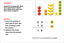
Math Example--Charts, Graphs, and Plots--Reading and Interpreting Scaled Graphs--Example 6 | Math Example--Charts, Graphs, and Plots-- Reading and Interpreting Scaled Graphs--Example 6
In this set of math examples, analyze the behavior of different scatterplots. This includes linear and quadratic models. |
Subtraction Facts to 100 and Data Analysis |
|
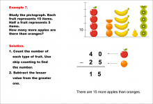
Math Example--Charts, Graphs, and Plots--Reading and Interpreting Scaled Graphs--Example 7 | Math Example--Charts, Graphs, and Plots-- Reading and Interpreting Scaled Graphs--Example 7
In this set of math examples, analyze the behavior of different scatterplots. This includes linear and quadratic models. |
Subtraction Facts to 100 and Data Analysis |
|
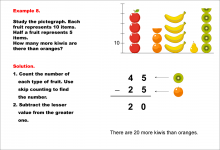
Math Example--Charts, Graphs, and Plots--Reading and Interpreting Scaled Graphs--Example 8 | Math Example--Charts, Graphs, and Plots-- Reading and Interpreting Scaled Graphs--Example 8
In this set of math examples, analyze the behavior of different scatterplots. This includes linear and quadratic models. |
Subtraction Facts to 100 and Data Analysis |
|
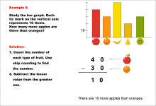
Math Example--Charts, Graphs, and Plots--Reading and Interpreting Scaled Graphs--Example 9 | Math Example--Charts, Graphs, and Plots-- Reading and Interpreting Scaled Graphs--Example 9
In this set of math examples, analyze the behavior of different scatterplots. This includes linear and quadratic models. |
Subtraction Facts to 100 and Data Analysis |
|
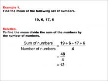
Math Example--Measures of Central Tendency--Mean: Example 1 | Math Example--Measures of Central Tendency--Mean: Example 1TopicMeasures of Central Tendency DescriptionThis example demonstrates how to calculate the mean of a dataset, a fundamental concept in statistics. The mean, often referred to as the average, is a measure of central tendency that provides insight into the typical value of a dataset. By visually presenting the calculation process, students can better grasp the concept and its application in real-world scenarios. |
Data Analysis |
|
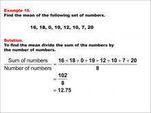
Math Example--Measures of Central Tendency--Mean: Example 10 | Math Example--Measures of Central Tendency--Mean: Example 10TopicMeasures of Central Tendency DescriptionThis example demonstrates the calculation of the mean for the numbers 16, 18, 0, 19, 12, 10, 7, and 20. The process involves summing all values (102) and dividing by the count of numbers (8), resulting in a mean of 12.75. This example highlights how the mean can provide a representative value for a dataset that includes both high and low numbers, including zero. |
Data Analysis |
|
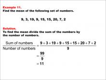
Math Example--Measures of Central Tendency--Mean: Example 11 | Math Example--Measures of Central Tendency--Mean: Example 11TopicMeasures of Central Tendency DescriptionThis example illustrates the calculation of the mean for the numbers 9, 3, 19, 9, 15, 15, 20, 7, and 2. The process involves summing all values (99) and dividing by the count of numbers (9), resulting in a mean of 11. This example demonstrates how the mean can provide a central value that represents a dataset with repeated numbers and a wide range of values. |
Data Analysis |
|
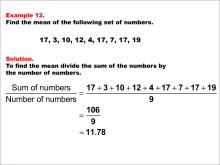
Math Example--Measures of Central Tendency--Mean: Example 12 | Math Example--Measures of Central Tendency--Mean: Example 12TopicMeasures of Central Tendency DescriptionThis example demonstrates the calculation of the mean for the numbers 17, 3, 10, 12, 4, 17, 7, 17, and 19. The process involves summing all values (106) and dividing by the count of numbers (9), resulting in a mean of approximately 11.78. This example showcases how the mean can provide a representative value for a dataset that includes repeated numbers and a wide range of values. |
Data Analysis |
|
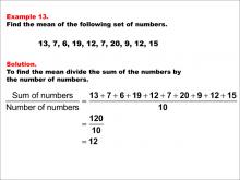
Math Example--Measures of Central Tendency--Mean: Example 13 | Math Example--Measures of Central Tendency--Mean: Example 13TopicMeasures of Central Tendency DescriptionThis example illustrates the calculation of the mean for the numbers 13, 7, 6, 19, 12, 7, 20, 9, 12, and 15. The process involves summing all values (120) and dividing by the count of numbers (10), resulting in a mean of 12. This example demonstrates how the mean can provide a central value that represents a dataset with repeated numbers and a wide range of values. |
Data Analysis |
|
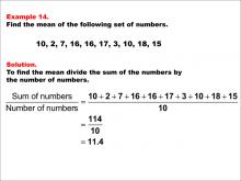
Math Example--Measures of Central Tendency--Mean: Example 14 | Math Example--Measures of Central Tendency--Mean: Example 14TopicMeasures of Central Tendency DescriptionThis example demonstrates the calculation of the mean for the numbers 10, 2, 7, 16, 16, 17, 3, 10, 18, and 15. The process involves summing all values (114) and dividing by the count of numbers (10), resulting in a mean of 11.4. This example showcases how the mean can provide a representative value for a dataset that includes repeated numbers and a wide range of values. |
Data Analysis |
|
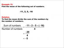
Math Example--Measures of Central Tendency--Mean: Example 15 | Math Example--Measures of Central Tendency--Mean: Example 15TopicMeasures of Central Tendency DescriptionThis example illustrates the calculation of the mean for the numbers -11, 2, 5, and -16. The process involves summing all values (-20) and dividing by the count of numbers (4), resulting in a mean of -5. This example is particularly important as it demonstrates how to handle negative numbers when calculating the mean, a concept that often challenges students. |
Data Analysis |
|
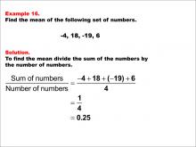
Math Example--Measures of Central Tendency--Mean: Example 16 | Math Example--Measures of Central Tendency--Mean: Example 16TopicMeasures of Central Tendency DescriptionThis example demonstrates the calculation of the mean for the numbers -4, 18, -19, and 6. The process involves summing all values (1) and dividing by the count of numbers (4), resulting in a mean of 0.25. This example is particularly interesting as it shows how positive and negative numbers can nearly balance each other out, resulting in a mean close to zero. |
Data Analysis |
|
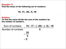
Math Example--Measures of Central Tendency--Mean: Example 17 | Math Example--Measures of Central Tendency--Mean: Example 17TopicMeasures of Central Tendency DescriptionThis example illustrates the calculation of the mean for the numbers 15, 17, -20, -5, and 18. The process involves summing all values (25) and dividing by the count of numbers (5), resulting in a mean of 5. This example is particularly instructive as it demonstrates how to handle a mix of positive and negative numbers, including some relatively large values in both directions. |
Data Analysis |
|
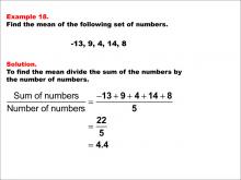
Math Example--Measures of Central Tendency--Mean: Example 18 | Math Example--Measures of Central Tendency--Mean: Example 18TopicMeasures of Central Tendency DescriptionThis example demonstrates the calculation of the mean for the numbers -13, 9, 4, 14, and 8. The process involves summing all values (22) and dividing by the count of numbers (5), resulting in a mean of 4.4. This example is particularly instructive as it shows how a single negative number can significantly impact the mean, even when most of the numbers are positive. |
Data Analysis |
|
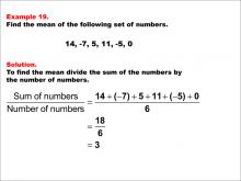
Math Example--Measures of Central Tendency--Mean: Example 19 | Math Example--Measures of Central Tendency--Mean: Example 19TopicMeasures of Central Tendency DescriptionThis example illustrates the calculation of the mean for the numbers 14, -7, 5, 11, -5, and 0. The process involves summing all values (18) and dividing by the count of numbers (6), resulting in a mean of 3. This example is particularly instructive as it demonstrates how to handle a mix of positive and negative numbers, including zero, in the calculation of the mean. |
Data Analysis |
|
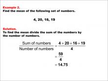
Math Example--Measures of Central Tendency--Mean: Example 2 | Math Example--Measures of Central Tendency--Mean: Example 2TopicMeasures of Central Tendency DescriptionThis example builds upon the concept of calculating the mean, introducing a slightly more complex dataset. It illustrates how the mean remains an effective measure of central tendency even as the numbers in the dataset become more varied. The visual representation helps students understand the step-by-step process of summing all values and dividing by the count of numbers. |
Data Analysis |

|
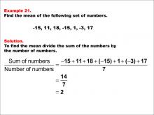
Math Example--Measures of Central Tendency--Mean: Example 20 | Math Example--Measures of Central Tendency--Mean: Example 20TopicMeasures of Central Tendency DescriptionThis example demonstrates the calculation of the mean for the numbers 19, -4, 11, 6, -6, and 1. The process involves summing all values (27) and dividing by the count of numbers (6), resulting in a mean of 4.5. This example is particularly instructive as it shows how positive and negative numbers interact in the calculation of the mean, resulting in a positive value despite the presence of negative numbers. |
Data Analysis |
|
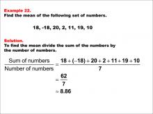
Math Example--Measures of Central Tendency--Mean: Example 21 | Math Example--Measures of Central Tendency--Mean: Example 21TopicMeasures of Central Tendency DescriptionThis example illustrates the calculation of the mean for the numbers -15, 11, 18, -15, 1, -3, and 17. The process involves summing all values (14) and dividing by the count of numbers (7), resulting in a mean of 2. This example is particularly instructive as it demonstrates how to handle a mix of positive and negative numbers, including repeated values, in the calculation of the mean. |
Data Analysis |
|
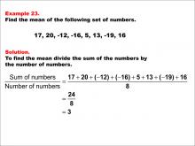
Math Example--Measures of Central Tendency--Mean: Example 22 | Math Example--Measures of Central Tendency--Mean: Example 22TopicMeasures of Central Tendency DescriptionThis example demonstrates the calculation of the mean for the numbers 18, -18, 20, 2, 11, 19, and 10. The process involves summing all values (62) and dividing by the count of numbers (7), resulting in a mean of approximately 8.86. This example is particularly instructive as it shows how a single large negative number can significantly impact the mean, even when most of the numbers are positive. |
Data Analysis |
|
Math Example--Measures of Central Tendency--Mean: Example 23 | Math Example--Measures of Central Tendency--Mean: Example 23TopicMeasures of Central Tendency DescriptionThis example illustrates the calculation of the mean for the numbers 17, 20, -12, -16, 5, 13, -19, and 16. The process involves summing all values (24) and dividing by the count of numbers (8), resulting in a mean of 3. This example is particularly instructive as it demonstrates how to handle a mix of positive and negative numbers with varying magnitudes in the calculation of the mean. |
Data Analysis |
|
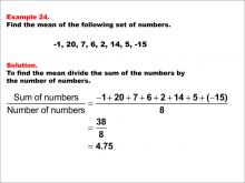
Math Example--Measures of Central Tendency--Mean: Example 24 | Math Example--Measures of Central Tendency--Mean: Example 24TopicMeasures of Central Tendency DescriptionThis example demonstrates the calculation of the mean for the numbers -1, 20, 7, 6, 2, 14, 5, and -15. The process involves summing all values (38) and dividing by the count of numbers (8), resulting in a mean of 4.75. This example is particularly instructive as it shows how a mix of positive and negative numbers, including some relatively large values in both directions, can interact to produce a mean that doesn't necessarily reflect the magnitude of the largest numbers in the set. |
Data Analysis |
|
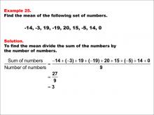
Math Example--Measures of Central Tendency--Mean: Example 25 | Math Example--Measures of Central Tendency--Mean: Example 25TopicMeasures of Central Tendency DescriptionThis example illustrates the calculation of the mean for the numbers -14, -3, 19, -19, 20, 15, -5, 14, and 0. The process involves summing all values (27) and dividing by the count of numbers (9), resulting in a mean of 3. This example is particularly instructive as it demonstrates how to handle a mix of positive and negative numbers, including zero, in the calculation of the mean. |
Data Analysis |
|
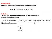
Math Example--Measures of Central Tendency--Mean: Example 26 | Math Example--Measures of Central Tendency--Mean: Example 26TopicMeasures of Central Tendency DescriptionThis example demonstrates the calculation of the mean for the numbers -10, -6, 19, 6, -6, 5, 6, 9, and 10. The process involves summing all values (33) and dividing by the count of numbers (9), resulting in a mean of approximately 3.67. This example is particularly instructive as it shows how positive and negative numbers interact in the calculation of the mean, resulting in a positive value despite the presence of negative numbers. |
Data Analysis |
|
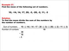
Math Example--Measures of Central Tendency--Mean: Example 27 | Math Example--Measures of Central Tendency--Mean: Example 27TopicMeasures of Central Tendency DescriptionThis example illustrates the calculation of the mean for the numbers 10, -14, 14, 17, 20, -3, -20, -2, 11, and -3. The process involves summing all values (30) and dividing by the count of numbers (10), resulting in a mean of 3. This example is particularly instructive as it demonstrates how to handle a mix of positive and negative numbers, including some relatively large values in both directions, in the calculation of the mean. |
Data Analysis |