
Illustrative Math Alignment: Grade 7 Unit 2
Introducing Proportional Relationships
Lesson 13: Two Graphs for Each Relationship
Use the following Media4Math resources with this Illustrative Math lesson.
| Thumbnail Image | Title | Body | Curriculum Nodes |
|---|---|---|---|
|
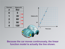
Math Clip Art--Applications of Linear Functions: Distance vs. Time 05 | Math Clip Art--Applications of Linear Functions: Distance vs. Time 05TopicLinear Functions DescriptionThis math clip art image continues the series on applications of linear functions, focusing on the distance-time relationship. It builds upon the previous graph by connecting the data points with a continuous line. The image emphasizes that because the car moves continuously, the linear function model is represented by this unbroken line, not just discrete points. |
Graphs of Linear Functions and Slope-Intercept Form |
|
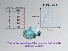
Math Clip Art--Applications of Linear Functions: Distance vs. Time 06 | Math Clip Art--Applications of Linear Functions: Distance vs. Time 06TopicLinear Functions DescriptionThis math clip art image is part of a series illustrating applications of linear functions, specifically modeling the relationship between distance and time. The image introduces the equation f(x) = 30x, which represents the function that models the car's movement. This equation encapsulates the linear relationship between time (x) and distance (f(x)) that has been explored in previous images. |
Graphs of Linear Functions and Slope-Intercept Form |
|
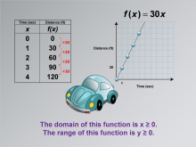
Math Clip Art--Applications of Linear Functions: Distance vs. Time 07 | Math Clip Art--Applications of Linear Functions: Distance vs. Time 07TopicLinear Functions DescriptionThis math clip art image continues the series on applications of linear functions, focusing on the domain and range of the distance-time function. The image emphasizes that the domain of this function is x ≥ 0, and the range is y ≥ 0. This representation helps students understand the practical constraints on the variables in real-world applications of linear functions. |
Graphs of Linear Functions and Slope-Intercept Form |
|
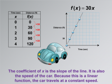
Math Clip Art--Applications of Linear Functions: Distance vs. Time 08 | Math Clip Art--Applications of Linear Functions: Distance vs. Time 08TopicLinear Functions DescriptionThis math clip art image continues the series on applications of linear functions, focusing on the relationship between distance and time. It builds upon previous illustrations by emphasizing that the coefficient of x in the equation f(x) = 30x represents both the slope of the line and the speed of the car. This image reinforces the concept that in a linear function, the rate of change remains constant throughout. |
Graphs of Linear Functions and Slope-Intercept Form |
|
Math Clip Art--Applications of Linear Functions: Distance vs. Time 09 | Math Clip Art--Applications of Linear Functions: Distance vs. Time 09TopicLinear Functions DescriptionThis math clip art image is part of a series illustrating applications of linear functions, with a focus on the distance-time relationship. It presents a new scenario with a car and an updated data table. The image likely introduces a different speed or starting point, allowing students to compare and contrast with the previous example and explore how changes in initial conditions affect the linear function. |
Graphs of Linear Functions and Slope-Intercept Form |
|
Math Clip Art--Applications of Linear Functions: Distance vs. Time 10 | Math Clip Art--Applications of Linear Functions: Distance vs. Time 10TopicLinear Functions DescriptionThis math clip art image concludes the series on applications of linear functions in the context of distance versus time relationships. It presents a linear graph corresponding to the data table introduced in the previous image. This visual representation allows students to see how the new scenario translates into a graphical form, reinforcing the connection between tabular data and its linear graph. |
Graphs of Linear Functions and Slope-Intercept Form |
|
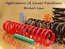
Math Clip Art--Applications of Linear Functions: Hooke's Law 01 | Math Clip Art--Applications of Linear Functions: Hooke's Law 01TopicLinear Functions DescriptionThis image serves as the title card for a series of illustrations demonstrating applications of linear functions, specifically focusing on Hooke's Law. The series, comprising eight images, explores the relationship between force and displacement in springs, showcasing how linear models can represent real-world phenomena. |
Graphs of Linear Functions, Slope-Intercept Form and Proportions |
|
|
Math Clip Art--Applications of Linear Functions: Hooke's Law 01 | Math Clip Art--Applications of Linear Functions: Hooke's Law 01TopicLinear Functions DescriptionThis image serves as the title card for a series of illustrations demonstrating applications of linear functions, specifically focusing on Hooke's Law. The series, comprising eight images, explores the relationship between force and displacement in springs, showcasing how linear models can represent real-world phenomena. |
Graphs of Linear Functions, Slope-Intercept Form and Proportions |
|
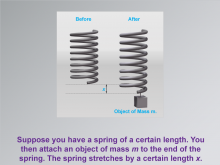
Math Clip Art--Applications of Linear Functions: Hooke's Law 02 | Math Clip Art--Applications of Linear Functions: Hooke's Law 02TopicLinear Functions DescriptionThis image is part of a series illustrating applications of linear functions, focusing on Hooke's Law. It depicts a spring before and after being stretched by a weight, visually representing the fundamental concept of Hooke's Law. The illustration shows a spring in its original state and then stretched by an object of mass m, extending by a length x. This visual representation helps students understand the relationship between the applied force (weight) and the resulting displacement of the spring, which forms the basis of the linear function in Hooke's Law. |
Graphs of Linear Functions, Slope-Intercept Form and Proportions |
|
|
Math Clip Art--Applications of Linear Functions: Hooke's Law 02 | Math Clip Art--Applications of Linear Functions: Hooke's Law 02TopicLinear Functions DescriptionThis image is part of a series illustrating applications of linear functions, focusing on Hooke's Law. It depicts a spring before and after being stretched by a weight, visually representing the fundamental concept of Hooke's Law. The illustration shows a spring in its original state and then stretched by an object of mass m, extending by a length x. This visual representation helps students understand the relationship between the applied force (weight) and the resulting displacement of the spring, which forms the basis of the linear function in Hooke's Law. |
Graphs of Linear Functions, Slope-Intercept Form and Proportions |
|
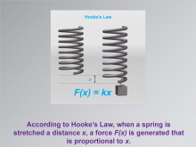
Math Clip Art--Applications of Linear Functions: Hooke's Law 03 | Math Clip Art--Applications of Linear Functions: Hooke's Law 03TopicLinear Functions DescriptionThis image is a continuation of the series on applications of linear functions, specifically illustrating Hooke's Law. It builds upon the previous image by introducing the mathematical equation F(x) = kx, which is the core of Hooke's Law. The illustration shows that when a spring is stretched a distance x, a force F(x) is generated that is proportional to x. This visual representation, combined with the equation, helps students understand the linear relationship between force and displacement in springs. |
Graphs of Linear Functions, Slope-Intercept Form and Proportions |
|
|
Math Clip Art--Applications of Linear Functions: Hooke's Law 03 | Math Clip Art--Applications of Linear Functions: Hooke's Law 03TopicLinear Functions DescriptionThis image is a continuation of the series on applications of linear functions, specifically illustrating Hooke's Law. It builds upon the previous image by introducing the mathematical equation F(x) = kx, which is the core of Hooke's Law. The illustration shows that when a spring is stretched a distance x, a force F(x) is generated that is proportional to x. This visual representation, combined with the equation, helps students understand the linear relationship between force and displacement in springs. |
Graphs of Linear Functions, Slope-Intercept Form and Proportions |
|
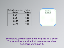
Math Clip Art--Applications of Linear Functions: Hooke's Law 04 | Math Clip Art--Applications of Linear Functions: Hooke's Law 04TopicLinear Functions DescriptionThis image is part of a series demonstrating applications of linear functions, focusing on Hooke's Law. It presents a practical application of the law by showing a data table alongside a weight scale, illustrating how Hooke's Law applies to everyday objects. |
Graphs of Linear Functions, Slope-Intercept Form and Proportions |
|
|
Math Clip Art--Applications of Linear Functions: Hooke's Law 04 | Math Clip Art--Applications of Linear Functions: Hooke's Law 04TopicLinear Functions DescriptionThis image is part of a series demonstrating applications of linear functions, focusing on Hooke's Law. It presents a practical application of the law by showing a data table alongside a weight scale, illustrating how Hooke's Law applies to everyday objects. |
Graphs of Linear Functions, Slope-Intercept Form and Proportions |
|
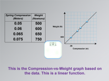
Math Clip Art--Applications of Linear Functions: Hooke's Law 05 | Math Clip Art--Applications of Linear Functions: Hooke's Law 05TopicLinear Functions DescriptionThis image is a continuation of the series on applications of linear functions, specifically illustrating Hooke's Law. It builds upon the previous image by presenting a graph of the data collected from the weight scale experiment. The illustration shows a Compression-vs-Weight graph based on the data from the weight scale. The graph displays a clear linear relationship, with data points connected by a straight line. This visual representation helps students see how the abstract concept of a linear function manifests in real-world data. |
Graphs of Linear Functions, Slope-Intercept Form and Proportions |
|
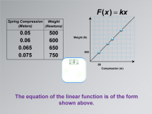
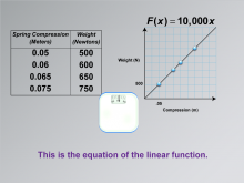
Math Clip Art--Applications of Linear Functions: Hooke's Law 06 | Math Clip Art--Applications of Linear Functions: Hooke's Law 06TopicLinear Functions DescriptionThis image is part of a series demonstrating applications of linear functions, specifically focusing on Hooke's Law. It builds upon the previous images by introducing the general form of the linear function equation that describes the relationship observed in the weight scale experiment. |
Graphs of Linear Functions, Slope-Intercept Form and Proportions |
|
|
Math Clip Art--Applications of Linear Functions: Hooke's Law 06 | Math Clip Art--Applications of Linear Functions: Hooke's Law 06TopicLinear Functions DescriptionThis image is part of a series demonstrating applications of linear functions, specifically focusing on Hooke's Law. It builds upon the previous images by introducing the general form of the linear function equation that describes the relationship observed in the weight scale experiment. |
Graphs of Linear Functions, Slope-Intercept Form and Proportions |
|
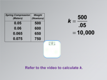
Math Clip Art--Applications of Linear Functions: Hooke's Law 07 | Math Clip Art--Applications of Linear Functions: Hooke's Law 07TopicLinear Functions DescriptionThis image is part of a series illustrating applications of linear functions, focusing on Hooke's Law. It builds upon previous images by demonstrating how to calculate the spring constant 'k' using the data collected from the weight scale experiment. Note: Here is the link to the video referenced: https://www.media4math.com/library/42143/asset-preview |
Graphs of Linear Functions, Slope-Intercept Form and Proportions |
|
|
Math Clip Art--Applications of Linear Functions: Hooke's Law 07 | Math Clip Art--Applications of Linear Functions: Hooke's Law 07TopicLinear Functions DescriptionThis image is part of a series illustrating applications of linear functions, focusing on Hooke's Law. It builds upon previous images by demonstrating how to calculate the spring constant 'k' using the data collected from the weight scale experiment. Note: Here is the link to the video referenced: https://www.media4math.com/library/42143/asset-preview |
Graphs of Linear Functions, Slope-Intercept Form and Proportions |
|
Math Clip Art--Applications of Linear Functions: Hooke's Law 08 | Math Clip Art--Applications of Linear Functions: Hooke's Law 08TopicLinear Functions DescriptionThis image represents the culmination of our exploration into applications of linear functions, specifically focusing on Hooke's Law. It serves as the final piece in a series of eight images, tying together all the concepts we've examined throughout this study of spring behavior and weight measurement. |
Graphs of Linear Functions, Slope-Intercept Form and Proportions |
|
|
Math Clip Art--Applications of Linear Functions: Hooke's Law 08 | Math Clip Art--Applications of Linear Functions: Hooke's Law 08TopicLinear Functions DescriptionThis image represents the culmination of our exploration into applications of linear functions, specifically focusing on Hooke's Law. It serves as the final piece in a series of eight images, tying together all the concepts we've examined throughout this study of spring behavior and weight measurement. |
Graphs of Linear Functions, Slope-Intercept Form and Proportions |

|
Math Clip Art--Applications of Linear Functions: Temperature Conversion 01 | Math Clip Art--Applications of Linear Functions: Temperature Conversion 01TopicLinear Functions DescriptionThis image serves as an introduction to a series of math clip art illustrations demonstrating applications of linear functions, specifically focusing on temperature conversion. The title card presents "Applications of Linear Functions: Temperature Conversion," setting the stage for a comprehensive exploration of how linear models can be used to convert between Celsius and Fahrenheit temperatures. |
Graphs of Linear Functions and Slope-Intercept Form |
|
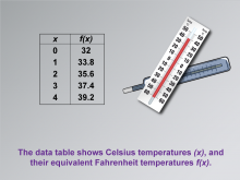
Math Clip Art--Applications of Linear Functions: Temperature Conversion 02 | Math Clip Art--Applications of Linear Functions: Temperature Conversion 02TopicLinear Functions DescriptionThis image is the second in a series illustrating applications of linear functions, focusing on temperature conversion. It presents a visual representation of thermometers alongside a data table that displays Celsius temperatures (x) and their corresponding Fahrenheit temperatures f(x). This pairing of visual and tabular data helps students connect the abstract concept of linear functions to the concrete idea of temperature scales. |
Graphs of Linear Functions and Slope-Intercept Form |
|
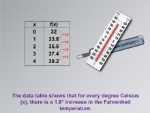
Math Clip Art--Applications of Linear Functions: Temperature Conversion 03 | Math Clip Art--Applications of Linear Functions: Temperature Conversion 03TopicLinear Functions DescriptionThis image is the third in a series demonstrating applications of linear functions through temperature conversion. It builds upon the previous image by highlighting a key observation: for every degree Celsius increase, there is a corresponding 1.8° increase in the Fahrenheit temperature. This insight is crucial in understanding the linear relationship between Celsius and Fahrenheit scales. |
Graphs of Linear Functions and Slope-Intercept Form |
|
Math Clip Art--Applications of Linear Functions: Temperature Conversion 04 | Math Clip Art--Applications of Linear Functions: Temperature Conversion 04TopicLinear Functions DescriptionThis image is part of a series illustrating applications of linear functions, focusing on temperature conversion. It builds upon previous images by introducing a data graph that visually represents the relationship between Celsius and Fahrenheit temperatures. The graph reinforces the key observation that for every degree Celsius increase, there is a corresponding 1.8° increase in the Fahrenheit temperature. |
Graphs of Linear Functions and Slope-Intercept Form |
|
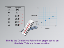
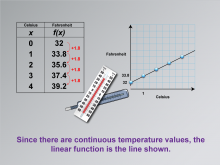
Math Clip Art--Applications of Linear Functions: Temperature Conversion 05 | Math Clip Art--Applications of Linear Functions: Temperature Conversion 05TopicLinear Functions DescriptionThis image continues the series on applications of linear functions in temperature conversion. It builds upon the previous graph by connecting the data points with a straight line. This visual representation emphasizes the continuous nature of temperature values and clearly illustrates the linear relationship between Celsius and Fahrenheit scales. |
Graphs of Linear Functions and Slope-Intercept Form |
|
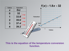
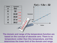
Math Clip Art--Applications of Linear Functions: Temperature Conversion 06 | Math Clip Art--Applications of Linear Functions: Temperature Conversion 06TopicLinear Functions DescriptionThis image is a crucial part of the series on applications of linear functions in temperature conversion. It introduces the mathematical equation f(x) = 1.8x + 32, which represents the temperature conversion function from Celsius to Fahrenheit. This equation is the culmination of the observations and data analysis from the previous images in the series. |
Graphs of Linear Functions and Slope-Intercept Form |
|
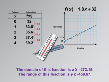
Math Clip Art--Applications of Linear Functions: Temperature Conversion 07 | Math Clip Art--Applications of Linear Functions: Temperature Conversion 07TopicLinear Functions DescriptionThis image continues the exploration of linear functions in temperature conversion by introducing the concepts of domain and range. It specifies that the domain of the temperature conversion function is x ≥ -273.15, and the range is y ≥ -459.67. These limits are crucial in understanding the real-world constraints on the mathematical model. |
Graphs of Linear Functions and Slope-Intercept Form |
|
Math Clip Art--Applications of Linear Functions: Temperature Conversion 08 | Math Clip Art--Applications of Linear Functions: Temperature Conversion 08TopicLinear Functions DescriptionThis image delves deeper into the concept of domain and range in the context of temperature conversion. It explains that the limits of the temperature function are based on the concept of absolute zero, the lowest theoretically possible temperature. This fundamental principle of physics determines the lower bounds of both the domain and range of the temperature conversion function. |
Graphs of Linear Functions and Slope-Intercept Form |

|
Math Clip Art--Applications of Linear Functions: Temperature Conversion 09 | Math Clip Art--Applications of Linear Functions: Temperature Conversion 09TopicLinear Functions DescriptionThis final image in the series on applications of linear functions in temperature conversion focuses on the significance of the coefficient of x in the linear equation. It emphasizes that this coefficient, 1.8 in the equation f(x) = 1.8x + 32, represents both the slope of the line and the temperature conversion rate. |
Graphs of Linear Functions and Slope-Intercept Form |
|
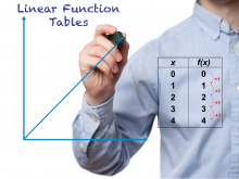
Math Clip Art--Linear Function Tables 01 | Math Clip Art--Linear Function Concepts--Linear Function Tables 01TopicLinear Functions DescriptionThis image is part of a series illustrating key concepts in linear functions, specifically focusing on linear function tables. It serves as a title card for a set of 10 clip art images that explore linear functions in tabular and graph form. This visual introduction sets the stage for understanding how linear functions can be represented and analyzed using tables. |
Graphs of Linear Functions and Slope-Intercept Form |
|
|
Math Clip Art--Linear Function Tables 01 | Math Clip Art--Linear Function Concepts--Linear Function Tables 01TopicLinear Functions DescriptionThis image is part of a series illustrating key concepts in linear functions, specifically focusing on linear function tables. It serves as a title card for a set of 10 clip art images that explore linear functions in tabular and graph form. This visual introduction sets the stage for understanding how linear functions can be represented and analyzed using tables. |
Graphs of Linear Functions and Slope-Intercept Form |
|
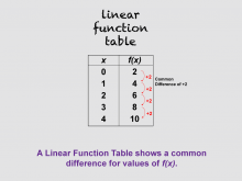
Math Clip Art--Linear Function Tables 02 | Math Clip Art--Linear Function Concepts--Linear Function Tables 02TopicLinear Functions DescriptionThis image is part of a series illustrating key concepts in linear functions, focusing on linear function tables. It presents a data table demonstrating that a linear function table shows a common difference for values of f(x). This visual representation helps students understand the fundamental characteristic of linear functions - the constant rate of change. |
Graphs of Linear Functions and Slope-Intercept Form |
|
|
Math Clip Art--Linear Function Tables 02 | Math Clip Art--Linear Function Concepts--Linear Function Tables 02TopicLinear Functions DescriptionThis image is part of a series illustrating key concepts in linear functions, focusing on linear function tables. It presents a data table demonstrating that a linear function table shows a common difference for values of f(x). This visual representation helps students understand the fundamental characteristic of linear functions - the constant rate of change. |
Graphs of Linear Functions and Slope-Intercept Form |
|
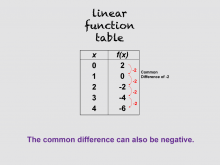
Math Clip Art--Linear Function Tables 03 | Math Clip Art--Linear Function Concepts--Linear Function Tables 03TopicLinear Functions DescriptionThis image is part of a series illustrating key concepts in linear functions, specifically linear function tables. It builds on the previous image by showing that the common difference in a linear function can also be negative. This concept is crucial for understanding decreasing linear functions and their representation in tabular form. |
Graphs of Linear Functions and Slope-Intercept Form |
|
|
Math Clip Art--Linear Function Tables 03 | Math Clip Art--Linear Function Concepts--Linear Function Tables 03TopicLinear Functions DescriptionThis image is part of a series illustrating key concepts in linear functions, specifically linear function tables. It builds on the previous image by showing that the common difference in a linear function can also be negative. This concept is crucial for understanding decreasing linear functions and their representation in tabular form. |
Graphs of Linear Functions and Slope-Intercept Form |
|
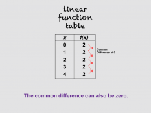
Math Clip Art--Linear Function Tables 04 | Math Clip Art--Linear Function Concepts--Linear Function Tables 04TopicLinear Functions DescriptionThis image is part of a series illustrating key concepts in linear functions, focusing on linear function tables. It presents a new version of the previous table, this time demonstrating that the common difference can also be zero. This concept introduces students to constant functions, a special case of linear functions where the output remains the same regardless of the input. |
Graphs of Linear Functions and Slope-Intercept Form |
|
|
Math Clip Art--Linear Function Tables 04 | Math Clip Art--Linear Function Concepts--Linear Function Tables 04TopicLinear Functions DescriptionThis image is part of a series illustrating key concepts in linear functions, focusing on linear function tables. It presents a new version of the previous table, this time demonstrating that the common difference can also be zero. This concept introduces students to constant functions, a special case of linear functions where the output remains the same regardless of the input. |
Graphs of Linear Functions and Slope-Intercept Form |
|
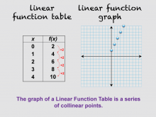
Math Clip Art--Linear Function Tables 05 | Math Clip Art--Linear Function Concepts--Linear Function Tables 05TopicLinear Functions DescriptionThis image is part of a series illustrating key concepts in linear functions, focusing on the relationship between linear function tables and graphs. It shows both a data table and a linear graph of data points, demonstrating that the graph of a Linear Function Table is a series of collinear points. This visual representation helps students connect tabular and graphical representations of linear functions. |
Graphs of Linear Functions and Slope-Intercept Form |
|
|
Math Clip Art--Linear Function Tables 05 | Math Clip Art--Linear Function Concepts--Linear Function Tables 05TopicLinear Functions DescriptionThis image is part of a series illustrating key concepts in linear functions, focusing on the relationship between linear function tables and graphs. It shows both a data table and a linear graph of data points, demonstrating that the graph of a Linear Function Table is a series of collinear points. This visual representation helps students connect tabular and graphical representations of linear functions. |
Graphs of Linear Functions and Slope-Intercept Form |
|
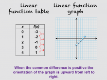
Math Clip Art--Linear Function Tables 06 | Math Clip Art--Linear Function Concepts--Linear Function Tables 06TopicLinear Functions DescriptionThis image is part of a series illustrating key concepts in linear functions, focusing on linear function tables and their corresponding graphs. It presents a variation of the previous image with a new set of data, demonstrating that when the common difference is positive, the orientation of the graph is upward from left to right. This helps students understand the concept of positive slope in linear functions. |
Graphs of Linear Functions and Slope-Intercept Form |
|
|
Math Clip Art--Linear Function Tables 06 | Math Clip Art--Linear Function Concepts--Linear Function Tables 06TopicLinear Functions DescriptionThis image is part of a series illustrating key concepts in linear functions, focusing on linear function tables and their corresponding graphs. It presents a variation of the previous image with a new set of data, demonstrating that when the common difference is positive, the orientation of the graph is upward from left to right. This helps students understand the concept of positive slope in linear functions. |
Graphs of Linear Functions and Slope-Intercept Form |
|
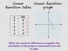
Math Clip Art--Linear Function Tables 07 | Math Clip Art--Linear Function Concepts--Linear Function Tables 07TopicLinear Functions DescriptionThis image is part of a series illustrating key concepts in linear functions, focusing on linear function tables and their corresponding graphs. It shows a variation of the previous image with a new set of data, demonstrating that when the common difference is negative, the orientation of the graph is downward from left to right. This helps students understand the concept of negative slope in linear functions. |
Graphs of Linear Functions and Slope-Intercept Form |
|
|
Math Clip Art--Linear Function Tables 07 | Math Clip Art--Linear Function Concepts--Linear Function Tables 07TopicLinear Functions DescriptionThis image is part of a series illustrating key concepts in linear functions, focusing on linear function tables and their corresponding graphs. It shows a variation of the previous image with a new set of data, demonstrating that when the common difference is negative, the orientation of the graph is downward from left to right. This helps students understand the concept of negative slope in linear functions. |
Graphs of Linear Functions and Slope-Intercept Form |
|
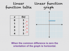
Math Clip Art--Linear Function Tables 08 | Math Clip Art--Linear Function Concepts--Linear Function Tables 08TopicLinear Functions DescriptionThis image is part of a series illustrating key concepts in linear functions, focusing on linear function tables and their corresponding graphs. It presents a variation of the previous image with a new set of data, showing that when the common difference is zero, the orientation of the graph is horizontal. This helps students understand the concept of zero slope in linear functions, also known as constant functions. |
Graphs of Linear Functions and Slope-Intercept Form |
|
|
Math Clip Art--Linear Function Tables 08 | Math Clip Art--Linear Function Concepts--Linear Function Tables 08TopicLinear Functions DescriptionThis image is part of a series illustrating key concepts in linear functions, focusing on linear function tables and their corresponding graphs. It presents a variation of the previous image with a new set of data, showing that when the common difference is zero, the orientation of the graph is horizontal. This helps students understand the concept of zero slope in linear functions, also known as constant functions. |
Graphs of Linear Functions and Slope-Intercept Form |
|
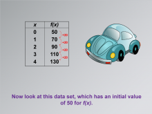
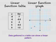
Math Clip Art--Linear Function Tables 09 | Math Clip Art--Linear Function Concepts--Linear Function Tables 09TopicLinear Functions DescriptionThis image is part of a series illustrating key concepts in linear functions, focusing on linear function tables. It shows a variation of the previous image with a new set of data, demonstrating that data gathered in a table can show a linear pattern. This concept helps students understand how to identify linear relationships from tabular data. |
Graphs of Linear Functions and Slope-Intercept Form |
|
|
Math Clip Art--Linear Function Tables 09 | Math Clip Art--Linear Function Concepts--Linear Function Tables 09TopicLinear Functions DescriptionThis image is part of a series illustrating key concepts in linear functions, focusing on linear function tables. It shows a variation of the previous image with a new set of data, demonstrating that data gathered in a table can show a linear pattern. This concept helps students understand how to identify linear relationships from tabular data. |
Graphs of Linear Functions and Slope-Intercept Form |
|
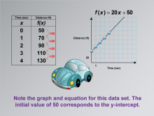
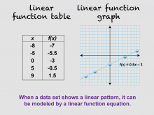
Math Clip Art--Linear Function Tables 10 | Math Clip Art--Linear Function Concepts--Linear Function Tables 10TopicLinear Functions DescriptionThis image is part of a series illustrating key concepts in linear functions, focusing on linear function tables and equations. It continues from the previous image, now including the equation f(x) = 0.5x - 3. This demonstrates that when a data set shows a linear pattern, it can be modeled by a linear function equation. This concept helps students understand the connection between tabular data and algebraic representations of linear functions. |
Graphs of Linear Functions and Slope-Intercept Form |
|
|
Math Clip Art--Linear Function Tables 10 | Math Clip Art--Linear Function Concepts--Linear Function Tables 10TopicLinear Functions DescriptionThis image is part of a series illustrating key concepts in linear functions, focusing on linear function tables and equations. It continues from the previous image, now including the equation f(x) = 0.5x - 3. This demonstrates that when a data set shows a linear pattern, it can be modeled by a linear function equation. This concept helps students understand the connection between tabular data and algebraic representations of linear functions. |
Graphs of Linear Functions and Slope-Intercept Form |