
Illustrative Math Alignment: Grade 6 Unit 8
Data Sets and Distributions
Lesson 12: Using Mean and MAD to Make Comparisons
Use the following Media4Math resources with this Illustrative Math lesson.
| Thumbnail Image | Title | Body | Curriculum Nodes |
|---|---|---|---|
|
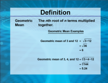
Video Definition 10--Rationals and Radicals--Geometric Mean (Spanish Audio) | Video Definition 10--Rationals and Radicals--Geometric Mean (Spanish Audio)
TopicRationals and Radicals DescriptionThe geometric mean is the nth root of the product of n terms. Examples include the geometric mean of 3 and 12, √(3 × 12) = 6, and the geometric mean of 3, 4, and 12, ∛(3 × 4 × 12) ≈ 5.24. Geometric mean connects multiplication and roots, commonly used in statistics, geometry, and proportional reasoning. This video includes Spanish audio and can be used with multilingual learners. |
Radical Expressions |

|
Video Definition 10--Rationals and Radicals--Geometric Mean | Video Definition 10--Rationals and Radicals--Geometric Mean
TopicRationals and Radicals DescriptionThe geometric mean is the nth root of the product of n terms. Examples include the geometric mean of 3 and 12, √(3 × 12) = 6, and the geometric mean of 3, 4, and 12, ∛(3 × 4 × 12) ≈ 5.24. Geometric mean connects multiplication and roots, commonly used in statistics, geometry, and proportional reasoning. |
Radical Expressions |
|
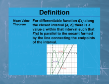
Definition--Calculus Topics--Mean Value Theorem | Definition--Calculus Topics--Mean Value TheoremTopicCalculus DefinitionThe Mean Value Theorem states that for a function f(x) that is continuous on [a,b] and differentiable on (a,b), there exists at least one c in (a,b) such that f'(c) = [f(b) - f(a)] / (b - a). DescriptionThe Mean Value Theorem is a fundamental result in calculus that connects the average rate of change of a function over an interval to its instantaneous rate of change at some point within that interval. It has important applications in both pure and applied mathematics, including optimization problems, approximation theory, and in proving other important theorems in calculus. |
Calculus Vocabulary |
|
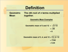
Definition--Rationals and Radicals--Geometric Mean | Geometric MeanTopicRationals and Radicals DefinitionThe geometric mean of two numbers is the square root of their product. DescriptionThe geometric mean is an example of using radical expressions to solve a problem. It provides a measure of central tendency that is particularly useful in situations where the numbers are multiplied together rather than added. In geometry, the geometric mean appears in various theorems and constructions. It is also used in finance and statistics to calculate average growth rates and to compare different sets of data. |
Radical Expressions |
|
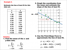
Math Example--Charts, Graphs, and Plots--Estimating the Line of Best Fit: Example 5 | Math Example--Charts, Graphs, and Plots-- Estimating the Line of Best Fit: Example 5
In this set of math examples, analyze the behavior of different scatterplots. This includes linear and quadratic models. |
Point-Slope Form, Slope-Intercept Form and Data Analysis |
|
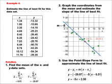
Math Example--Charts, Graphs, and Plots--Estimating the Line of Best Fit: Example 4 | Math Example--Charts, Graphs, and Plots-- Estimating the Line of Best Fit: Example 4
In this set of math examples, analyze the behavior of different scatterplots. This includes linear and quadratic models. |
Point-Slope Form, Slope-Intercept Form and Data Analysis |
|
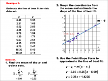
Math Example--Charts, Graphs, and Plots--Estimating the Line of Best Fit: Example 3 | Math Example--Charts, Graphs, and Plots-- Estimating the Line of Best Fit: Example 3
In this set of math examples, analyze the behavior of different scatterplots. This includes linear and quadratic models. |
Point-Slope Form, Slope-Intercept Form and Data Analysis |
|
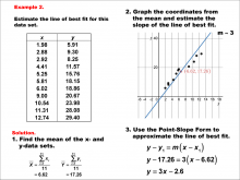
Math Example--Charts, Graphs, and Plots--Estimating the Line of Best Fit: Example 2 | Math Example--Charts, Graphs, and Plots-- Estimating the Line of Best Fit: Example 2
In this set of math examples, analyze the behavior of different scatterplots. This includes linear and quadratic models. |
Point-Slope Form, Slope-Intercept Form and Data Analysis |
|
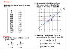
Math Example--Charts, Graphs, and Plots--Estimating the Line of Best Fit: Example 1 | Math Example--Charts, Graphs, and Plots-- Estimating the Line of Best Fit: Example 1
In this set of math examples, analyze the behavior of different scatterplots. This includes linear and quadratic models. |
Slope-Intercept Form and Data Analysis |

|
INSTRUCTIONAL RESOURCE: Algebra Application: Why Are Receipts So Long? | INSTRUCTIONAL RESOURCE: Algebra Application: Why Are Receipts So Long?
In this Algebra Application, students gather data to study the lengths of paper receipts. They also learn to estimate the total number of receipts produced worldwide using industry data. From this they can study the environmental impact of having to produce so many paper receipts. The math topics covered include: Measures of central tendency (specifically the mean), Scientific notation, Rates, Converting different units. The culminating activity is for students to make a persuasive case to retailers about finding alternatives to paper receipts, using the data they gathered and analyzed. This is a great back-to-school activity for middle school or high school students. A relevant real-world application allows them to review math concepts. |
Laws of Exponents and Data Analysis |
|
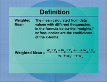
Definition--Measures of Central Tendency--Weighted Mean | Weighted MeanTopicStatistics DefinitionThe weighted mean is the average of a data set where each value is multiplied by a weight reflecting its importance. DescriptionThe weighted mean is used when different data points contribute unequally to the final average. It is commonly applied in finance to calculate portfolio returns, in education to compute weighted grades, and in various fields where data points have different levels of significance. The weighted mean provides a more accurate representation of data by considering the relative importance of each value. |
Data Analysis |
|
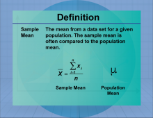
Definition--Measures of Central Tendency--Sample Mean | Sample MeanTopicStatistics DefinitionThe sample mean is the average of a sample, calculated by summing the sample values and dividing by the sample size. DescriptionThe sample mean is a measure of central tendency that provides an estimate of the population mean based on a sample. It is widely used in statistics for making inferences about populations from samples, playing a crucial role in hypothesis testing and confidence interval estimation. The sample mean is used in fields such as economics, biology, and psychology to analyze data and draw conclusions about larger populations. |
Data Analysis |
|
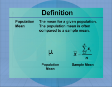
Definition--Measures of Central Tendency--Population Mean | Population MeanTopicStatistics DefinitionThe population mean is a measure of central tendency that provides an average representation of a set of data. DescriptionThe Population Mean is an important concept in statistics, used to summarize data effectively. It is meant to represent the mean for a given statistic for an entire population. For example, the mean length of a salmon. |
Data Analysis |
|
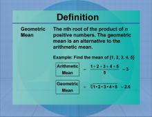
Definition--Measures of Central Tendency--Geometric Mean | Geometric MeanTopicStatistics DefinitionThe geometric mean is the nth root of the product of n numbers, used to calculate average rates of growth. DescriptionThe geometric mean is particularly useful in finance and economics for calculating compound interest and growth rates. Unlike the arithmetic mean, it is appropriate for data sets with values that are multiplicatively related. For example, the geometric mean of 2, 8, and 32 is calculated as (2 × 8 × 32)1/3 = 8. In mathematics, the geometric mean is essential for understanding exponential growth and decay. |
Data Analysis |
|
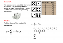
Math Example--Measures of Central Tendency--Mean of a Probability Distribution--Example 1 | Math Example--Measures of Central Tendency--Mean of a Probability Distribution--Example 1TopicMeasures of Central Tendency DescriptionThis example demonstrates the calculation of the mean for a probability distribution of a fair six-sided die. The probability of each outcome (1 to 6) is equally 1/6. The mean is calculated by multiplying each possible outcome by its probability and summing the results. For this fair die, the mean is determined to be 3.5. |
Data Analysis |
|
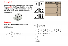
Math Example--Measures of Central Tendency--Mean of a Probability Distribution--Example 2 | Math Example--Measures of Central Tendency--Mean of a Probability Distribution--Example 2TopicMeasures of Central Tendency DescriptionThis example illustrates the calculation of the mean for a probability distribution of an unfair six-sided die. Unlike a fair die, the probabilities are not equally distributed, with a higher probability (2/6) for rolling a 1. The mean is calculated using the same method as before, resulting in approximately 2.83. |
Data Analysis |

|
Math Example--Measures of Central Tendency--Mean of a Probability Distribution--Example 3 | Math Example--Measures of Central Tendency--Mean of a Probability Distribution--Example 3TopicMeasures of Central Tendency DescriptionThis example demonstrates the calculation of the mean for another unfair six-sided die. In this case, the probability of rolling a 1 is even higher (3/6), while some numbers have a probability of 0. The mean is calculated using the same method, resulting in 2.5. |
Data Analysis |
|
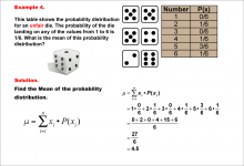
Math Example--Measures of Central Tendency--Mean of a Probability Distribution--Example 4 | Math Example--Measures of Central Tendency--Mean of a Probability Distribution--Example 4TopicMeasures of Central Tendency DescriptionThis example illustrates the calculation of the mean for an unfair six-sided die where the number 5 has a significantly higher probability (3/6) than other numbers. The mean is calculated using the same method as previous examples, resulting in 4.5. |
Data Analysis |
|
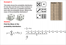
Math Example--Measures of Central Tendency--Mean of a Probability Distribution--Example 5 | Math Example--Measures of Central Tendency--Mean of a Probability Distribution--Example 5TopicMeasures of Central Tendency DescriptionThis example demonstrates the calculation of the mean for the probability distribution of the sum when rolling two fair dice. There are 11 possible outcomes (2 to 12), each with its own probability. The mean is calculated using the same method as previous examples, resulting in 7. |
Data Analysis |
|
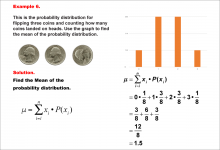
Math Example--Measures of Central Tendency--Mean of a Probability Distribution--Example 6 | Math Example--Measures of Central Tendency--Mean of a Probability Distribution--Example 6TopicMeasures of Central Tendency DescriptionThis example illustrates the calculation of the mean for the probability distribution of the number of heads when flipping three fair coins. The possible outcomes are 0, 1, 2, or 3 heads, each with its own probability. The mean is calculated using the same method as previous examples, resulting in 1.5. |
Data Analysis |
|
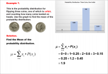
Math Example--Measures of Central Tendency--Mean of a Probability Distribution--Example 7 | Math Example--Measures of Central Tendency--Mean of a Probability Distribution--Example 7TopicMeasures of Central Tendency DescriptionThis example demonstrates the calculation of the mean for the probability distribution of the number of heads when flipping three coins, one of which is unfair. The possible outcomes are 0, 1, 2, or 3 heads, but the probabilities are skewed due to the unfair coin. The mean is calculated using the same method as previous examples, resulting in 1.9. |
Data Analysis |

|
Math Example--Measures of Central Tendency--Sample Mean--Example 1 | Math Example--Measures of Central Tendency--Sample Mean--Example 1TopicMeasures of Central Tendency DescriptionThis example demonstrates the calculation of the sample mean for a group of 30 trout. The image displays a table showing the lengths of these trout, along with the formula for calculating the sample mean. The population of adult trout has a mean length of 15 inches with a standard deviation of 2. The sample mean is calculated by summing all the lengths (472.22 inches) and dividing by the number of trout (30), resulting in a sample mean of 15.74 inches. |
Data Analysis |
|
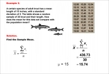
Math Example--Measures of Central Tendency--Sample Mean--Example 2 | Math Example--Measures of Central Tendency--Sample Mean--Example 2TopicMeasures of Central Tendency DescriptionThis example presents another calculation of the sample mean for a group of 30 trout. The image shows a table with the lengths of these trout and the formula for the sample mean. The population of adult trout has a mean length of 15 inches with a standard deviation of 2. The sample mean is computed by adding all the lengths (436.73 inches) and dividing by the number of trout (30), yielding a sample mean of 14.56 inches. |
Data Analysis |
|
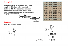
Math Example--Measures of Central Tendency--Sample Mean--Example 3 | Math Example--Measures of Central Tendency--Sample Mean--Example 3TopicMeasures of Central Tendency DescriptionThis example illustrates the calculation of the sample mean for a group of 40 trout. The image displays a table showing the lengths of these trout, along with the formula for calculating the sample mean. The population of adult trout has a mean length of 15 inches with a standard deviation of 2. The sample mean is calculated by summing all the lengths (615.86 inches) and dividing by the number of trout (40), resulting in a sample mean of 15.39 inches. |
Data Analysis |

|
Math Example--Measures of Central Tendency--Sample Mean--Example 4 | Math Example--Measures of Central Tendency--Sample Mean--Example 4TopicMeasures of Central Tendency DescriptionThis example demonstrates the calculation of the sample mean for a group of 30 macaws. The image shows a table with the wingspans of these macaws and the formula for calculating the sample mean. The population of adult macaws has an average wingspan of 48 inches with a standard deviation of 6. The sample mean is computed by summing all the wingspans (1432.28 inches) and dividing by the number of macaws (30), yielding a sample mean of 47.74 inches. |
Data Analysis |
|
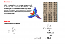
Math Example--Measures of Central Tendency--Sample Mean--Example 5 | Math Example--Measures of Central Tendency--Sample Mean--Example 5TopicMeasures of Central Tendency DescriptionThis example illustrates the calculation of the sample mean for another group of 30 macaws. The image displays a table showing the wingspans of these macaws, along with the formula for calculating the sample mean. The population of adult macaws has an average wingspan of 48 inches with a standard deviation of 6. The sample mean is calculated by summing all the wingspans (1398.02 inches) and dividing by the number of macaws (30), resulting in a sample mean of 46.6 inches. |
Data Analysis |
|
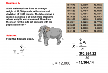
Math Example--Measures of Central Tendency--Sample Mean--Example 6 | Math Example--Measures of Central Tendency--Sample Mean--Example 6TopicMeasures of Central Tendency DescriptionThis example demonstrates the calculation of the sample mean for a group of 30 adult male elephants. The image shows a table with the weights of these elephants and the formula for calculating the sample mean. The population of adult male elephants has an average weight of 12,000 pounds with a standard deviation of 1,500 pounds. The sample mean is computed by summing all the weights (370,924.22 pounds) and dividing by the number of elephants (30), yielding a sample mean of 12,364.14 pounds. |
Data Analysis |
|
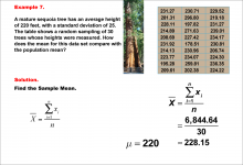
Math Example--Measures of Central Tendency--Sample Mean--Example 7 | Math Example--Measures of Central Tendency--Sample Mean--Example 7TopicMeasures of Central Tendency DescriptionThis example demonstrates the calculation of the sample mean for a group of 30 mature sequoia trees. The image presents a table showing the heights of these trees, along with the formula for computing the sample mean. The population of mature sequoia trees has an average height of 220 feet with a standard deviation of 25 feet. By summing all the heights (6,844.64 feet) and dividing by the number of trees (30), we obtain a sample mean of 228.15 feet. |
Data Analysis |
|
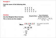
Math Example--Measures of Central Tendency--Weighted Mean--Example 1 | Math Example--Measures of Central Tendency--Weighted Mean--Example 1TopicMeasures of Central Tendency DescriptionThis example demonstrates the calculation of a weighted mean for a data set consisting of the values 6, 9, and 7, with weights of 4, 5, and 6 respectively. The weighted mean is computed using the formula: (4 * 6 + 5 * 9 + 6 * 7) / (4 + 5 + 6), resulting in a final answer of 7.4. |
Data Analysis |
|
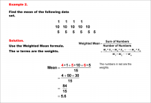
Math Example--Measures of Central Tendency--Weighted Mean--Example 2 | Math Example--Measures of Central Tendency--Weighted Mean--Example 2TopicMeasures of Central Tendency DescriptionThis example illustrates the calculation of a weighted mean for a data set containing the values 1, 10, and 5, with weights of 4, 5, and 6 respectively. The weighted mean is computed using the formula: (4 * 1 + 5 * 10 + 6 * 5) / (4 + 5 + 6), resulting in a final answer of 5.6. |
Data Analysis |
|
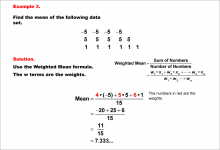
Math Example--Measures of Central Tendency--Weighted Mean--Example 3 | Math Example--Measures of Central Tendency--Weighted Mean--Example 3TopicMeasures of Central Tendency DescriptionThis example demonstrates the calculation of a weighted mean for a data set containing negative and positive values: -5, 5, and 1, with weights of 4, 5, and 6 respectively. The weighted mean is computed using the formula: (4 * -5 + 5 * 5 + 6 * 1) / (4 + 5 + 6), resulting in a final answer of approximately 0.733. |
Data Analysis |
|
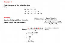
Math Example--Measures of Central Tendency--Weighted Mean--Example 4 | Math Example--Measures of Central Tendency--Weighted Mean--Example 4TopicMeasures of Central Tendency DescriptionThis example illustrates the calculation of a weighted mean for a data set containing mostly negative values: -3, 2, and -5, with weights of 4, 3, and 5 respectively. The weighted mean is computed using the formula: (4 * -3 + 3 * 2 + 5 * -5) / (4 + 3 + 5), resulting in a final answer of approximately -2.133. |
Data Analysis |
|
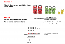
Math Example--Measures of Central Tendency--Weighted Mean--Example 5 | Math Example--Measures of Central Tendency--Weighted Mean--Example 5TopicMeasures of Central Tendency DescriptionThis example demonstrates the calculation of a weighted mean in a real-world context, using kettlebells of different weights: 32, 24, and 16 pounds, with quantities of 4, 6, and 3 respectively. The weighted mean is computed using the formula: (4 * 32 + 6 * 24 + 3 * 16) / (4 + 6 + 3), resulting in an average weight of 24.62 pounds. |
Data Analysis |
|
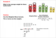
Math Example--Measures of Central Tendency--Weighted Mean--Example 6 | Math Example--Measures of Central Tendency--Weighted Mean--Example 6TopicMeasures of Central Tendency DescriptionThis example illustrates another real-world application of weighted mean, using kettlebells of different weights: 32, 24, and 16 pounds, with quantities of 5, 7, and 4 respectively. The weighted mean is computed using the formula: (5 * 32 + 7 * 24 + 4 * 16) / (5 + 7 + 4), resulting in an average weight of 24.5 pounds. |
Data Analysis |
|
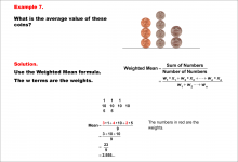
Math Example--Measures of Central Tendency--Weighted Mean--Example 7 | Math Example--Measures of Central Tendency--Weighted Mean--Example 7TopicMeasures of Central Tendency DescriptionThis example demonstrates the calculation of a weighted mean using coins of different values: pennies (1 cent), nickels (5 cents), and dimes (10 cents), with quantities of 3, 2, and 4 respectively. The weighted mean is computed using the formula: (3 * 1 + 2 * 5 + 4 * 10) / (3 + 2 + 4), resulting in an average value of approximately 5.56 cents. |
Data Analysis |
|
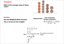
Math Example--Measures of Central Tendency--Weighted Mean--Example 8 | Math Example--Measures of Central Tendency--Weighted Mean--Example 8TopicMeasures of Central Tendency DescriptionThis example illustrates the calculation of a weighted mean using a collection of coins with different values. The image shows pennies, nickels, dimes, and quarters stacked in columns, representing quantities of 4, 3, 5, and 2 respectively. The weighted mean is computed using the formula: (4 * 1 + 3 * 5 + 5 * 10 + 2 * 25) / (4 + 3 + 5 + 2), resulting in an average value of 8.5 cents. |
Data Analysis |
|
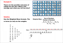
Math Example--Measures of Central Tendency--Weighted Mean--Example 9 | Math Example--Measures of Central Tendency--Weighted Mean--Example 9TopicMeasures of Central Tendency DescriptionThis example demonstrates the calculation of a weighted mean in the context of probability, specifically finding the average sum when rolling two fair dice. The image displays a grid showing all possible outcomes of rolling two dice, with sums ranging from 2 to 12. The frequencies of each sum are highlighted in red, serving as the weights in the weighted mean calculation. The weighted mean is computed using the formula: (2 * 1 + 3 * 2 + 4 * 3 + 5 * 4 + 6 * 5 + 7 * 6 + 8 * 5 + 9 * 4 + 10 * 3 + 11 * 2 + 12 * 1) / 36, resulting in an average sum of 7. |
Data Analysis |
|
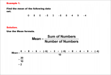
Math Example--Measures of Central Tendency--Mean of Data That Includes Negative Numbers--Example 1 | Math Example--Measures of Central Tendency--Mean of Data That Includes Negative Numbers--Example 1TopicMeasures of Central Tendency DescriptionThis math example demonstrates the calculation of the mean for a data set that includes negative numbers: 0, 8, 5, -5, 3, -8, 8, 4, 9, -4. The example emphasizes the step-by-step process of finding the mean, showing how to handle both positive and negative values in the calculation. |
Data Analysis |

|
Math Example--Measures of Central Tendency--Mean of Data That Includes Negative Numbers--Example 2 | Math Example--Measures of Central Tendency--Mean of Data That Includes Negative Numbers--Example 2TopicMeasures of Central Tendency DescriptionThis example illustrates the calculation of the mean for a dataset containing both positive and negative numbers: 7, 4, 1, 1, -1, -2, 9, 4, -9, -4. The step-by-step process shows how to sum all values, including negative ones, and divide by the total number of data points to find the mean. |
Data Analysis |
|
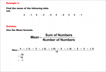
Math Example--Measures of Central Tendency--Mean of Data That Includes Negative Numbers--Example 3 | Math Example--Measures of Central Tendency--Mean of Data That Includes Negative Numbers--Example 3TopicMeasures of Central Tendency DescriptionThis example demonstrates the calculation of the mean for a dataset that includes negative numbers and zeros: 4, -1, 0, -2, -9, 0, -6, 5, 0, -1. The step-by-step process illustrates how to sum all values, including negatives and zeros, and divide by the total number of data points to determine the mean. |
Data Analysis |

|
Math Example--Measures of Central Tendency--Mean of Data That Includes Negative Numbers--Example 4 | Math Example--Measures of Central Tendency--Mean of Data That Includes Negative Numbers--Example 4TopicMeasures of Central Tendency DescriptionThis example illustrates the calculation of the mean for a dataset containing both positive and negative numbers: -3, 8, 2, 1, 3, -6, -9, 3, -4. The step-by-step process demonstrates how to sum all values, including negative ones, and divide by the total number of data points to find the mean. |
Data Analysis |
|
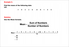
Math Example--Measures of Central Tendency--Mean of Data That Includes Negative Numbers--Example 5 | Math Example--Measures of Central Tendency--Mean of Data That Includes Negative Numbers--Example 5TopicMeasures of Central Tendency DescriptionThis example demonstrates the calculation of the mean for a dataset that includes both positive and negative numbers: -1, 9, 3, 3, 6, -8, 8, 1, 4, 5. The step-by-step process shows how to sum all values, including negative ones, and divide by the total number of data points to determine the mean. |
Data Analysis |
|
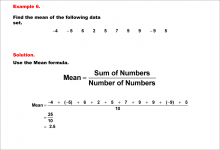
Math Example--Measures of Central Tendency--Mean of Data That Includes Negative Numbers--Example 6 | Math Example--Measures of Central Tendency--Mean of Data That Includes Negative Numbers--Example 6TopicMeasures of Central Tendency DescriptionThis example illustrates the calculation of the mean for a dataset containing both positive and negative numbers: -4, -5, 6, 2, 5, 7, 9, 9, -9, 5. The step-by-step process demonstrates how to sum all values, including negative ones, and divide by the total number of data points to find the mean. |
Data Analysis |

|
Math Example--Measures of Central Tendency--Mean of Data That Includes Negative Numbers--Example 7 | Math Example--Measures of Central Tendency--Mean of Data That Includes Negative Numbers--Example 7TopicMeasures of Central Tendency DescriptionThis example demonstrates the calculation of the mean for a dataset that includes negative numbers and zero: -4, 0, 2, 9, -2, -3, -5, 10, -7, 5. The step-by-step process illustrates how to sum all values, including negatives and zero, and divide by the total number of data points to determine the mean. |
Data Analysis |

|
Math Example--Measures of Central Tendency--Mean of Data That Includes Negative Numbers--Example 8 | Math Example--Measures of Central Tendency--Mean of Data That Includes Negative Numbers--Example 8TopicMeasures of Central Tendency DescriptionThis image shows a math example calculating the mean of a data set. The numbers are: 4, 8, -6, -6, 6, -3, 4, -8, -6, -8. The solution uses the mean formula. Example 8 demonstrates finding the mean of the data set. The mean is calculated by summing all numbers and dividing by the count of numbers, resulting in (-15) / (10) = -1.5. |
Data Analysis |

|
Math Example--Measures of Central Tendency--Mean of Data That Includes Negative Numbers--Example 9 | Math Example--Measures of Central Tendency--Mean of Data That Includes Negative Numbers--Example 9TopicMeasures of Central Tendency DescriptionThe image shows Example 9, illustrating how to find the mean of a data set using the mean formula. This example demonstrates finding the mean of the data set: -8, -9, 10, -2, 3, -2, -8, -3, 2, 5. The calculation is shown step-by-step: Mean = Sum / Count. The sum of all numbers (-8 + (-9) + 10 + (-2) + 3 + (-2) + (-8) + (-3) + 2 + 5) is divided by the count of numbers (10), resulting in -12 / 10 = -1.2. |
Data Analysis |
|
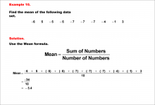
Math Example--Measures of Central Tendency--Mean of Data That Includes Negative Numbers--Example 10 | Math Example--Measures of Central Tendency--Mean of Data That Includes Negative Numbers--Example 10TopicMeasures of Central Tendency DescriptionThe image shows Example 10, demonstrating how to calculate the mean for a different set of numbers. This example illustrates finding the mean of the data set: -6, 5, -5, -5, -7, -7, -4, -1, 3. The calculation is presented step-by-step: Mean = Sum / Count. The sum of all numbers (-6 + 5 + (-5) + (-5) + (-7) + (-7) + (-4) + (-1) + 3) is divided by the count of numbers (10), resulting in -34 / 10 = -3.4. |
Data Analysis |
|
Interactive Math Game--DragNDrop--Measures of Central Tendency--Mean | Interactive Math Game--DragNDrop Math--Measures of Central Tendency--Mean
In this drag-and-drop game, have students practice their skills at calculating the mean of a data set. This game generates thousands of different combinations, offering an ideal opportunity for skill review in a game format. This is part of a collection of math games and interactives. To see the complete collection of the games, click on this link. Note: The download is the teacher's guide.Related ResourcesTo see additional resources on this topic, click on the Related Resources tab. |
Data Analysis |

|
Closed Captioned Video: Mean of a Data List | Closed Captioned Video: Mean of a Data List
In this TI Nspire tutorial, the Spreadsheet and Calculator windows are used to find the mean of a data list. This video supports the TI-Nspire Clickpad and Touchpad. This Mini-Tutorial Video includes a worksheet. . |
Data Analysis |

|
Video Transcript: TI-Nspire Mini-Tutorial: Finding the Mean of a Data List | Video Transcript: TI-Nspire Mini-Tutorial: Finding the Mean of a Data List
This is the transcript for the TI-Nspire Mini-Tutorial entitled, Finding the Mean of a Data List. This is part of a collection of video transcripts for the video tutorial series on using the TI-Nspire Graphing Calculator. To see the complete collection of transcripts, click on this link. Note: The download is a PDF file. Video Transcript LibraryTo see the complete collection of video transcriptsy, click on this link. |
Data Analysis |