Illustrative Math Alignment: Grade 6 Unit 8

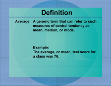
Topic

Statistics

Definition

The average is a measure of central tendency, calculated by dividing the sum of values by their count.

Description

In statistics, the average is crucial for analyzing data sets, revealing trends, and providing insight into overall performance. It’s applicable in various fields, from school grades to business metrics. For example, if a student scores 80, 90, and 100 on three exams, the average can be calculated as follows: Average = (80 + 90 + 100) / 3 = 90. The average is essential in math education as it forms a foundational concept for more advanced statistical analyses.

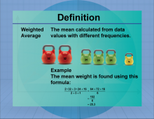
Topic

Statistics

Definition

A weighted average is an average that takes into account the relative importance of each value, calculated by multiplying each value by its weight and summing the results.

Description

The weighted average is used when different data points contribute unequally to the final average. It is commonly applied in finance to calculate portfolio returns, in education to compute weighted grades, and in various fields where data points have different levels of significance. The weighted average provides a more accurate representation of data by considering the relative importance of each value.

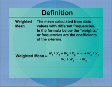
Topic

Statistics

Definition

The weighted mean is the average of a data set where each value is multiplied by a weight reflecting its importance.

Description

The weighted mean is used when different data points contribute unequally to the final average. It is commonly applied in finance to calculate portfolio returns, in education to compute weighted grades, and in various fields where data points have different levels of significance. The weighted mean provides a more accurate representation of data by considering the relative importance of each value.

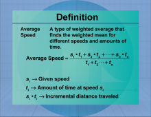
Topic

Statistics

Definition

Average speed is the total distance traveled divided by the total time taken.

Description

This concept finds application in areas such as physics, transport, and everyday scenarios like calculating travel time. For example, if a car travels 300 km in 3 hours, the average speed is Average Speed = 300 km / 3 hours = 100 km/h. Understanding average speed is key in mathematics as it helps contextualize rate and distance problems in real-life situations.

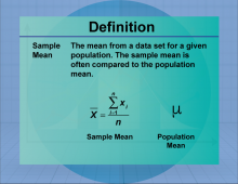
Topic

Statistics

Definition

The sample mean is the average of a sample, calculated by summing the sample values and dividing by the sample size.

Description

The sample mean is a measure of central tendency that provides an estimate of the population mean based on a sample. It is widely used in statistics for making inferences about populations from samples, playing a crucial role in hypothesis testing and confidence interval estimation. The sample mean is used in fields such as economics, biology, and psychology to analyze data and draw conclusions about larger populations.

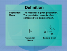
Topic

Statistics

Definition

The population mean is a measure of central tendency that provides an average representation of a set of data.

Description

The Population Mean is an important concept in statistics, used to summarize data effectively. It is meant to represent the mean for a given statistic for an entire population. For example, the mean length of a salmon.

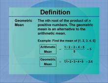
Topic

Statistics

Definition

The geometric mean is the nth root of the product of n numbers, used to calculate average rates of growth.

Description

The geometric mean is particularly useful in finance and economics for calculating compound interest and growth rates. Unlike the arithmetic mean, it is appropriate for data sets with values that are multiplicatively related. For example, the geometric mean of 2, 8, and 32 is calculated as (2 × 8 × 32)1/3 = 8. In mathematics, the geometric mean is essential for understanding exponential growth and decay.

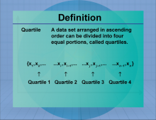
Topic

Statistics

Definition

Quartiles divide a ranked data set into four equal parts.

Description

Quartiles are used to summarize data by dividing it into four parts, each representing a quarter of the data set. They provide insight into the spread and center of data, helping to identify the distribution and variability. Quartiles are used in box plots to visually represent data distribution, making them valuable in fields such as finance and research for analyzing data trends.

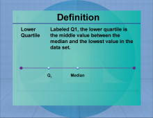
Topic

Statistics

Definition

The lower quartile (Q1) is the median of the lower half of a data set, representing the 25th percentile.

Description

The lower quartile is a measure of position, indicating the value below which 25% of the data falls. It is used in conjunction with other quartiles to understand the distribution and spread of data. In real-world applications, the lower quartile is used in finance to assess the performance of investments and in education to evaluate student achievement levels.

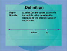
Topic

Statistics

Definition

The upper quartile (Q3) is the median of the upper half of a data set, representing the 75th percentile.

Description

The upper quartile is a measure of position that indicates the value below which 75% of the data falls. It is used in conjunction with other quartiles to understand the distribution and spread of data. In real-world applications, the upper quartile is used in finance to assess investment performance and in education to evaluate student achievement levels.

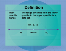
Topic

Statistics

Definition

The interquartile range (IQR) is the range between the first and third quartiles, representing the middle 50% of a data set.

Description

The IQR is a measure of statistical dispersion, indicating the spread of the central portion of a data set. It is particularly useful for identifying outliers and understanding the variability of data. In real-world applications, the IQR is used in finance to assess investment risks and in quality control to monitor process stability.

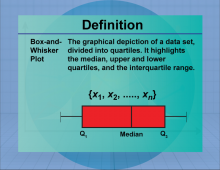
Topic

Statistics

Definition

A box-and-whisker plot is a graphical representation of data that displays the distribution through quartiles.

Description

Box-and-whisker plots are useful for visualizing the spread and skewness of a data set, highlighting the median, quartiles, and potential outliers. They are particularly valuable in comparing distributions across different groups. In real-world applications, box plots are used in quality control processes and in analyzing survey data to identify trends and anomalies.

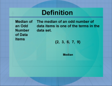
Topic

Statistics

Definition

The median of an odd data set is one of the terms in the data set.

Description

The Median is the middle term of a data set. If the data set consists of an odd number of terms, no matter how many terms there are, the Median will be the middle term of that set.

In mathematics education, understanding median of an odd data set is crucial as it lays the foundation for more advanced statistical concepts. It allows students to grasp the significance of data analysis and interpretation. In classes, students often perform exercises calculating the mean of sets, which enhances their understanding of averaging techniques.

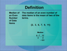
Topic

Statistics

Definition

The median of an even data set is the mean of two of the terms.

Description

The Median is the middle term of a data set. If the data set consists of an even number of terms, then the Median won't be one of ther terms in the set. In such a case the Median is the Mean of the two middle terms. 

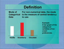
Topic

Statistics

Definition

The mode of categorical data is the most frequent item in a categorical data set.

Description

The Mode of Categorical Data is useful for finding the most frequent data item used with non-numerical data. For example, preferences for discrete characteristics can result in a mode.

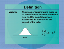
Topic

Statistics

Definition

Variance is a measure of the dispersion of a set of values, calculated as the average of the squared deviations from the mean.

Description

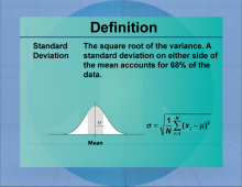
Variance quantifies the degree of spread in a data set, providing insight into the variability of data points around the mean. It is a fundamental concept in statistics, used in fields such as finance, research, and engineering to assess risk and variability. A high variance indicates greater dispersion, while a low variance suggests that data points are closer to the mean.

Topic

Statistics

Definition

Standard deviation is a measure of the amount of variation or dispersion in a set of values.

Description

Standard deviation quantifies the degree of variation in a data set, indicating how much individual data points deviate from the mean. It is a crucial statistic for understanding the spread of data and is widely used in fields such as finance, research, and quality control to assess variability and risk. A low standard deviation indicates that data points are close to the mean, while a high standard deviation suggests greater variability.

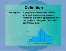
Topic

Statistics

Definition

A histogram is a graphical representation of data distribution using bars of different heights.

Description

Histograms are used to visualize the frequency distribution of continuous data, making it easier to identify patterns and trends. They are widely used in fields such as economics, biology, and engineering to analyze data distributions and detect anomalies. In mathematics, histograms are essential for understanding probability distributions and statistical inference.

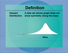
Topic

Statistics

Definition

A skewed distribution is a probability distribution that is not symmetric, with data tending to cluster more on one side.

Description

Skewed distributions occur when data is not evenly distributed around the mean, resulting in a longer tail on one side. Skewness can be positive (right-skewed) or negative (left-skewed), affecting the interpretation of data and statistical measures such as the mean and median. 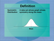Skewed distributions are common in real-world data, such as income levels and test scores, where extreme values can influence the overall distribution.

Topic

Statistics

Definition

A symmetric distribution is a probability distribution where the left and right sides are mirror images of each other.

Description

Symmetric distributions are characterized by data that is evenly distributed around the mean, resulting in a balanced, mirror-image shape. The most common symmetric distribution is the normal distribution, which is widely used in statistics for modeling natural phenomena. Symmetric distributions are important for statistical inference, as many statistical tests assume data is symmetrically distributed.

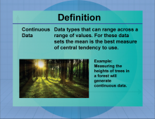
Topic

Statistics

Definition

Continuous data is numerical data that can take any value within a range.

Description

Continuous data is vital for representing measurements such as height, weight, and temperature, which can assume an infinite number of values within a given range. In real-world applications, continuous data is used in fields like engineering, physics, and economics to model and predict outcomes. Understanding continuous data is essential for performing calculations involving integrals and derivatives in calculus.

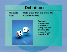
Topic

Statistics

Definition

Discrete data consists of countable values, often represented by whole numbers.

Description

Discrete data is commonly used in situations where data points are distinct and separate, such as the number of students in a class or the number of cars in a parking lot. It is crucial for fields like computer science, where discrete structures and algorithms are fundamental. In mathematics, discrete data is used in probability theory and combinatorics, helping to solve problems involving permutations and combinations.

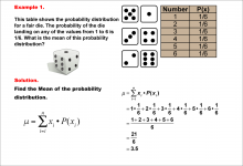
Topic

Measures of Central Tendency

Description

This example demonstrates the calculation of the mean for a probability distribution of a fair six-sided die. The probability of each outcome (1 to 6) is equally 1/6. The mean is calculated by multiplying each possible outcome by its probability and summing the results. For this fair die, the mean is determined to be 3.5.

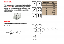
Topic

Measures of Central Tendency

Description

This example illustrates the calculation of the mean for a probability distribution of an unfair six-sided die. Unlike a fair die, the probabilities are not equally distributed, with a higher probability (2/6) for rolling a 1. The mean is calculated using the same method as before, resulting in approximately 2.83.

Topic

Measures of Central Tendency

Description

This example demonstrates the calculation of the mean for another unfair six-sided die. In this case, the probability of rolling a 1 is even higher (3/6), while some numbers have a probability of 0. The mean is calculated using the same method, resulting in 2.5.

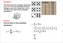
Topic

Measures of Central Tendency

Description

This example illustrates the calculation of the mean for an unfair six-sided die where the number 5 has a significantly higher probability (3/6) than other numbers. The mean is calculated using the same method as previous examples, resulting in 4.5.

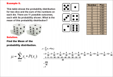
Topic

Measures of Central Tendency

Description

This example demonstrates the calculation of the mean for the probability distribution of the sum when rolling two fair dice. There are 11 possible outcomes (2 to 12), each with its own probability. The mean is calculated using the same method as previous examples, resulting in 7.

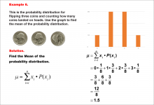
Topic

Measures of Central Tendency

Description

This example illustrates the calculation of the mean for the probability distribution of the number of heads when flipping three fair coins. The possible outcomes are 0, 1, 2, or 3 heads, each with its own probability. The mean is calculated using the same method as previous examples, resulting in 1.5.

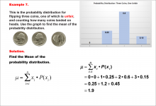
Topic

Measures of Central Tendency

Description

This example demonstrates the calculation of the mean for the probability distribution of the number of heads when flipping three coins, one of which is unfair. The possible outcomes are 0, 1, 2, or 3 heads, but the probabilities are skewed due to the unfair coin. The mean is calculated using the same method as previous examples, resulting in 1.9.

Topic

Measures of Central Tendency

Description

This example demonstrates the calculation of the sample mean for a group of 30 trout. The image displays a table showing the lengths of these trout, along with the formula for calculating the sample mean. The population of adult trout has a mean length of 15 inches with a standard deviation of 2. The sample mean is calculated by summing all the lengths (472.22 inches) and dividing by the number of trout (30), resulting in a sample mean of 15.74 inches.

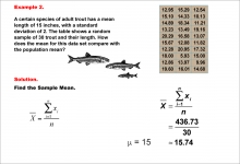
Topic

Measures of Central Tendency

Description

This example presents another calculation of the sample mean for a group of 30 trout. The image shows a table with the lengths of these trout and the formula for the sample mean. The population of adult trout has a mean length of 15 inches with a standard deviation of 2. The sample mean is computed by adding all the lengths (436.73 inches) and dividing by the number of trout (30), yielding a sample mean of 14.56 inches.

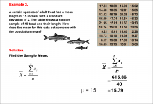
Topic

Measures of Central Tendency

Description

This example illustrates the calculation of the sample mean for a group of 40 trout. The image displays a table showing the lengths of these trout, along with the formula for calculating the sample mean. The population of adult trout has a mean length of 15 inches with a standard deviation of 2. The sample mean is calculated by summing all the lengths (615.86 inches) and dividing by the number of trout (40), resulting in a sample mean of 15.39 inches.

Topic

Measures of Central Tendency

Description

This example demonstrates the calculation of the sample mean for a group of 30 macaws. The image shows a table with the wingspans of these macaws and the formula for calculating the sample mean. The population of adult macaws has an average wingspan of 48 inches with a standard deviation of 6. The sample mean is computed by summing all the wingspans (1432.28 inches) and dividing by the number of macaws (30), yielding a sample mean of 47.74 inches.

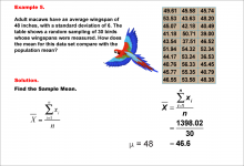
Topic

Measures of Central Tendency

Description

This example illustrates the calculation of the sample mean for another group of 30 macaws. The image displays a table showing the wingspans of these macaws, along with the formula for calculating the sample mean. The population of adult macaws has an average wingspan of 48 inches with a standard deviation of 6. The sample mean is calculated by summing all the wingspans (1398.02 inches) and dividing by the number of macaws (30), resulting in a sample mean of 46.6 inches.

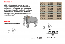
Topic

Measures of Central Tendency

Description

This example demonstrates the calculation of the sample mean for a group of 30 adult male elephants. The image shows a table with the weights of these elephants and the formula for calculating the sample mean. The population of adult male elephants has an average weight of 12,000 pounds with a standard deviation of 1,500 pounds. The sample mean is computed by summing all the weights (370,924.22 pounds) and dividing by the number of elephants (30), yielding a sample mean of 12,364.14 pounds.

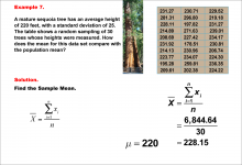
Topic

Measures of Central Tendency

Description

This example demonstrates the calculation of the sample mean for a group of 30 mature sequoia trees. The image presents a table showing the heights of these trees, along with the formula for computing the sample mean. The population of mature sequoia trees has an average height of 220 feet with a standard deviation of 25 feet. By summing all the heights (6,844.64 feet) and dividing by the number of trees (30), we obtain a sample mean of 228.15 feet.

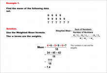
Topic

Measures of Central Tendency

Description

This example demonstrates the calculation of a weighted mean for a data set consisting of the values 6, 9, and 7, with weights of 4, 5, and 6 respectively. The weighted mean is computed using the formula: (4 * 6 + 5 * 9 + 6 * 7) / (4 + 5 + 6), resulting in a final answer of 7.4.

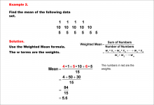
Topic

Measures of Central Tendency

Description

This example illustrates the calculation of a weighted mean for a data set containing the values 1, 10, and 5, with weights of 4, 5, and 6 respectively. The weighted mean is computed using the formula: (4 * 1 + 5 * 10 + 6 * 5) / (4 + 5 + 6), resulting in a final answer of 5.6.

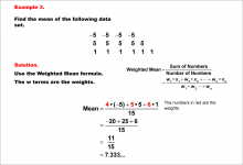
Topic

Measures of Central Tendency

Description

This example demonstrates the calculation of a weighted mean for a data set containing negative and positive values: -5, 5, and 1, with weights of 4, 5, and 6 respectively. The weighted mean is computed using the formula: (4 * -5 + 5 * 5 + 6 * 1) / (4 + 5 + 6), resulting in a final answer of approximately 0.733.

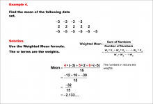
Topic

Measures of Central Tendency

Description

This example illustrates the calculation of a weighted mean for a data set containing mostly negative values: -3, 2, and -5, with weights of 4, 3, and 5 respectively. The weighted mean is computed using the formula: (4 * -3 + 3 * 2 + 5 * -5) / (4 + 3 + 5), resulting in a final answer of approximately -2.133.

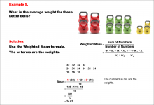
Topic

Measures of Central Tendency

Description

This example demonstrates the calculation of a weighted mean in a real-world context, using kettlebells of different weights: 32, 24, and 16 pounds, with quantities of 4, 6, and 3 respectively. The weighted mean is computed using the formula: (4 * 32 + 6 * 24 + 3 * 16) / (4 + 6 + 3), resulting in an average weight of 24.62 pounds.

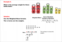
Topic

Measures of Central Tendency

Description

This example illustrates another real-world application of weighted mean, using kettlebells of different weights: 32, 24, and 16 pounds, with quantities of 5, 7, and 4 respectively. The weighted mean is computed using the formula: (5 * 32 + 7 * 24 + 4 * 16) / (5 + 7 + 4), resulting in an average weight of 24.5 pounds.

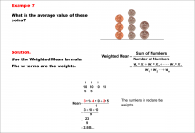
Topic

Measures of Central Tendency

Description

This example demonstrates the calculation of a weighted mean using coins of different values: pennies (1 cent), nickels (5 cents), and dimes (10 cents), with quantities of 3, 2, and 4 respectively. The weighted mean is computed using the formula: (3 * 1 + 2 * 5 + 4 * 10) / (3 + 2 + 4), resulting in an average value of approximately 5.56 cents.

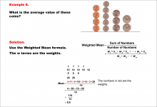
Topic

Measures of Central Tendency

Description

This example illustrates the calculation of a weighted mean using a collection of coins with different values. The image shows pennies, nickels, dimes, and quarters stacked in columns, representing quantities of 4, 3, 5, and 2 respectively. The weighted mean is computed using the formula: (4 * 1 + 3 * 5 + 5 * 10 + 2 * 25) / (4 + 3 + 5 + 2), resulting in an average value of 8.5 cents.

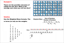
Topic

Measures of Central Tendency

Description

This example demonstrates the calculation of a weighted mean in the context of probability, specifically finding the average sum when rolling two fair dice. The image displays a grid showing all possible outcomes of rolling two dice, with sums ranging from 2 to 12. The frequencies of each sum are highlighted in red, serving as the weights in the weighted mean calculation. The weighted mean is computed using the formula: (2 * 1 + 3 * 2 + 4 * 3 + 5 * 4 + 6 * 5 + 7 * 6 + 8 * 5 + 9 * 4 + 10 * 3 + 11 * 2 + 12 * 1) / 36, resulting in an average sum of 7.

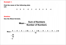
Topic

Measures of Central Tendency

Description

This math example demonstrates the calculation of the mean for a data set that includes negative numbers: 0, 8, 5, -5, 3, -8, 8, 4, 9, -4. The example emphasizes the step-by-step process of finding the mean, showing how to handle both positive and negative values in the calculation.

Topic

Measures of Central Tendency

Description

This example illustrates the calculation of the mean for a dataset containing both positive and negative numbers: 7, 4, 1, 1, -1, -2, 9, 4, -9, -4. The step-by-step process shows how to sum all values, including negative ones, and divide by the total number of data points to find the mean.

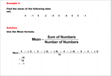
Topic

Measures of Central Tendency

Description

This example demonstrates the calculation of the mean for a dataset that includes negative numbers and zeros: 4, -1, 0, -2, -9, 0, -6, 5, 0, -1. The step-by-step process illustrates how to sum all values, including negatives and zeros, and divide by the total number of data points to determine the mean.

Topic

Measures of Central Tendency

Description

This example illustrates the calculation of the mean for a dataset containing both positive and negative numbers: -3, 8, 2, 1, 3, -6, -9, 3, -4. The step-by-step process demonstrates how to sum all values, including negative ones, and divide by the total number of data points to find the mean.

Topic

Measures of Central Tendency

Description

This example demonstrates the calculation of the mean for a dataset that includes both positive and negative numbers: -1, 9, 3, 3, 6, -8, 8, 1, 4, 5. The step-by-step process shows how to sum all values, including negative ones, and divide by the total number of data points to determine the mean.