
Illustrative Math Alignment: Grade 7 Unit 2
Introducing Proportional Relationships
Lesson 11: Interpreting Graphs of Proportional Relationships
Use the following Media4Math resources with this Illustrative Math lesson.
| Thumbnail Image | Title | Body | Curriculum Nodes |
|---|---|---|---|
|
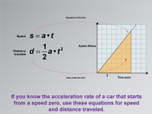
Math Clip Art--Applications of Linear and Quadratic Functions: Speed and Acceleration 17 | Math Clip Art--Applications of Linear and Quadratic Functions: Speed and Acceleration 17TopicQuadratics DescriptionThis image displays a graph with speed versus time, highlighting the equation of the line and the area under it. It emphasizes using these equations when acceleration starts from zero. If you know the acceleration rate of a car that starts from speed zero, use these equations for speed and distance traveled. The use of math clip art provides visual clarity in understanding how equations model motion from rest. Teacher's Script: "Notice these equations—how do they help us understand acceleration from rest?" |
Graphs of Linear Functions and Graphs of Quadratic Functions |
|
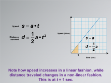
Math Clip Art--Applications of Linear and Quadratic Functions: Speed and Acceleration 18 | Math Clip Art--Applications of Linear and Quadratic Functions: Speed and Acceleration 18TopicQuadratics DescriptionThis image shows a graph with speed on the y-axis and time on the x-axis. The equations for speed and distance traveled are given as s = a⋅t and d = 1/2at2. The graph illustrates how speed increases linearly, while distance traveled follows a non-linear path. Math clip art like this helps students understand the difference between linear and quadratic relationships in real-world contexts. |
Graphs of Linear Functions and Graphs of Quadratic Functions |

|
Math Clip Art--Applications of Linear and Quadratic Functions: Speed and Acceleration 18 | Math Clip Art--Applications of Linear and Quadratic Functions: Speed and Acceleration 18TopicQuadratics DescriptionThis image shows a graph with speed on the y-axis and time on the x-axis. The equations for speed and distance traveled are given as s = a⋅t and d = 1/2at2. The graph illustrates how speed increases linearly, while distance traveled follows a non-linear path. Math clip art like this helps students understand the difference between linear and quadratic relationships in real-world contexts. |
Graphs of Linear Functions and Graphs of Quadratic Functions |
|
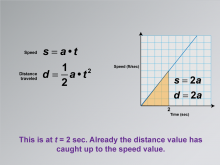
Math Clip Art--Applications of Linear and Quadratic Functions: Speed and Acceleration 19 | Math Clip Art--Applications of Linear and Quadratic Functions: Speed and Acceleration 19TopicQuadratics DescriptionThis image shows a graph similar to the previous image but at t = 2 seconds. The equations are updated to s = 2a and d = 2a, indicating that distance has caught up with speed. The use of math clip art provides visual clarity in understanding dynamic interactions between speed and distance over time. Teacher's Script: "At two seconds, notice how distance catches up to speed. What does this mean for our understanding of motion?" |
Graphs of Linear Functions and Graphs of Quadratic Functions |

|
Math Clip Art--Applications of Linear and Quadratic Functions: Speed and Acceleration 19 | Math Clip Art--Applications of Linear and Quadratic Functions: Speed and Acceleration 19TopicQuadratics DescriptionThis image shows a graph similar to the previous image but at t = 2 seconds. The equations are updated to s = 2a and d = 2a, indicating that distance has caught up with speed. The use of math clip art provides visual clarity in understanding dynamic interactions between speed and distance over time. Teacher's Script: "At two seconds, notice how distance catches up to speed. What does this mean for our understanding of motion?" |
Graphs of Linear Functions and Graphs of Quadratic Functions |
|
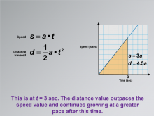
Math Clip Art--Applications of Linear and Quadratic Functions: Speed and Acceleration 20 | Math Clip Art--Applications of Linear and Quadratic Functions: Speed and Acceleration 20TopicQuadratics DescriptionThis image depicts a graph of speed versus time with no initial velocity. The equations shown are s = a⋅t for speed and d = 1/2at2 for distance traveled. At t = 3 seconds, the graph highlights that distance outpaces speed. The use of math clip art helps students visualize how distance can grow faster than speed under certain conditions. Teacher's Script: "At three seconds, see how distance outpaces speed? Let's explore why this happens." |
Graphs of Linear Functions and Graphs of Quadratic Functions |

|
Math Clip Art--Applications of Linear and Quadratic Functions: Speed and Acceleration 20 | Math Clip Art--Applications of Linear and Quadratic Functions: Speed and Acceleration 20TopicQuadratics DescriptionThis image depicts a graph of speed versus time with no initial velocity. The equations shown are s = a⋅t for speed and d = 1/2at2 for distance traveled. At t = 3 seconds, the graph highlights that distance outpaces speed. The use of math clip art helps students visualize how distance can grow faster than speed under certain conditions. Teacher's Script: "At three seconds, see how distance outpaces speed? Let's explore why this happens." |
Graphs of Linear Functions and Graphs of Quadratic Functions |
|
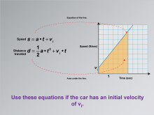
Math Clip Art--Applications of Linear and Quadratic Functions: Speed and Acceleration 21 | Math Clip Art--Applications of Linear and Quadratic Functions: Speed and Acceleration 21TopicQuadratics DescriptionThis image shows a graph with a line representing speed as a function of time, with initial velocity. The equations for speed are s = a⋅t+vi and for distance traveled are d= 1/2at2 +vi •t. The graph illustrates the area under the line, indicating distance. The use of math clip art provides students with visual tools to understand how initial velocity affects motion over time. Teacher's Script: "Notice how initial velocity changes the graph. How does this affect our calculations for distance?" |
Graphs of Linear Functions and Graphs of Quadratic Functions |

|
Math Clip Art--Applications of Linear and Quadratic Functions: Speed and Acceleration 21 | Math Clip Art--Applications of Linear and Quadratic Functions: Speed and Acceleration 21TopicQuadratics DescriptionThis image shows a graph with a line representing speed as a function of time, with initial velocity. The equations for speed are s = a⋅t+vi and for distance traveled are d= 1/2at2 +vi •t. The graph illustrates the area under the line, indicating distance. The use of math clip art provides students with visual tools to understand how initial velocity affects motion over time. Teacher's Script: "Notice how initial velocity changes the graph. How does this affect our calculations for distance?" |
Graphs of Linear Functions and Graphs of Quadratic Functions |

|
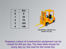
Math Clip Art--Applications of Linear Functions: Cost vs. Time 01 | Math Clip Art--Applications of Linear Functions: Cost vs. Time 01TopicLinear Functions |
Graphs of Linear Functions and Slope-Intercept Form |
|
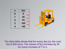
Math Clip Art--Applications of Linear Functions: Cost vs. Time 02 | Math Clip Art--Applications of Linear Functions: Cost vs. Time 02TopicLinear Functions |
Graphs of Linear Functions and Slope-Intercept Form |
|
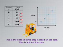
Math Clip Art--Applications of Linear Functions: Cost vs. Time 03 | Math Clip Art--Applications of Linear Functions: Cost vs. Time 03TopicLinear Functions |
Graphs of Linear Functions and Slope-Intercept Form |
|
Math Clip Art--Applications of Linear Functions: Cost vs. Time 04 | Math Clip Art--Applications of Linear Functions: Cost vs. Time 04TopicLinear Functions |
Graphs of Linear Functions and Slope-Intercept Form |
|
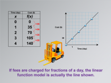
Math Clip Art--Applications of Linear Functions: Cost vs. Time 05 | Math Clip Art--Applications of Linear Functions: Cost vs. Time 05TopicLinear Functions |
Graphs of Linear Functions and Slope-Intercept Form |
|
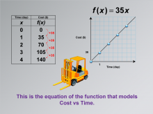
Math Clip Art--Applications of Linear Functions: Cost vs. Time 06 | Math Clip Art--Applications of Linear Functions: Cost vs. Time 06TopicLinear Functions |
Graphs of Linear Functions and Slope-Intercept Form |
|
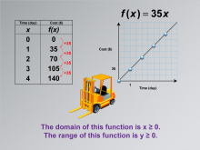
Math Clip Art--Applications of Linear Functions: Cost vs. Time 07 | Math Clip Art--Applications of Linear Functions: Cost vs. Time 07TopicLinear Functions DescriptionThis math clip art image is the seventh in a series dedicated to illustrating applications of linear functions, specifically focusing on building a linear function model for equipment rental costs. The image builds upon the previous one by introducing the concepts of domain and range in the context of the rental cost function. It continues to feature the construction equipment scenario, emphasizing the practical constraints on the function's input and output values. |
Graphs of Linear Functions and Slope-Intercept Form |
|
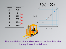
Math Clip Art--Applications of Linear Functions: Cost vs. Time 08 | Math Clip Art--Applications of Linear Functions: Cost vs. Time 08TopicLinear Functions DescriptionThis math clip art image is the eighth in a series exploring applications of linear functions, focusing on building a linear function model for equipment rental costs. The image emphasizes the relationship between the coefficient of x in the linear equation, the slope of the line in the graph, and the real-world rental rate. It continues to feature the construction equipment scenario, providing a concrete context for understanding these mathematical concepts. |
Graphs of Linear Functions and Slope-Intercept Form |
|
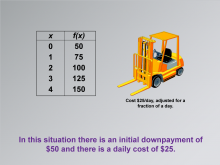
Math Clip Art--Applications of Linear Functions: Cost vs. Time 09 | Math Clip Art--Applications of Linear Functions: Cost vs. Time 09TopicLinear Functions |
Graphs of Linear Functions and Slope-Intercept Form |
|
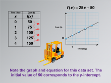
Math Clip Art--Applications of Linear Functions: Cost vs. Time 10 | Math Clip Art--Applications of Linear Functions: Cost vs. Time 10TopicLinear Functions |
Graphs of Linear Functions and Slope-Intercept Form |

|
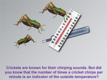
Math Clip Art--Applications of Linear Functions: Cricket Chirps 01 | Math Clip Art--Applications of Linear Functions: Cricket Chirps 01TopicLinear Functions DescriptionThis image introduces the topic Applications of Linear Functions: Cricket Chirps and sets the stage for understanding the relationship between the number of cricket chirps and outside temperature. It serves as a title card for a series of images exploring how linear functions can model real-world scenarios, specifically the connection between cricket chirps and outdoor temperature. |
Graphs of Linear Functions and Slope-Intercept Form |
|
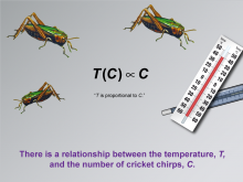
Math Clip Art--Applications of Linear Functions: Cricket Chirps 02 | Math Clip Art--Applications of Linear Functions: Cricket Chirps 02TopicLinear Functions DescriptionThis image in the series on applications of linear functions introduces the concept of crickets as nature's thermometers. It visually represents how the frequency of cricket chirps can indicate outside temperature, setting the foundation for exploring the linear relationship between these variables. |
Graphs of Linear Functions and Slope-Intercept Form |
|
Math Clip Art--Applications of Linear Functions: Cricket Chirps 03 | Math Clip Art--Applications of Linear Functions: Cricket Chirps 03TopicLinear Functions DescriptionThis image in the series on applications of linear functions illustrates the direct relationship between temperature (T) and the number of cricket chirps (C). It visually represents how these two variables are connected, laying the groundwork for developing a linear function model. |
Graphs of Linear Functions and Slope-Intercept Form |
|
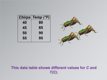
Math Clip Art--Applications of Linear Functions: Cricket Chirps 04 | Math Clip Art--Applications of Linear Functions: Cricket Chirps 04TopicLinear Functions DescriptionThis image presents a data table showing different values for cricket chirps (C) and corresponding temperatures (T). It's a crucial step in building a linear function model, as it provides the raw data from which the relationship will be derived. |
Graphs of Linear Functions and Slope-Intercept Form |
|
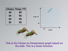
Math Clip Art--Applications of Linear Functions: Cricket Chirps 05 | Math Clip Art--Applications of Linear Functions: Cricket Chirps 05TopicLinear Functions DescriptionThis image in the series on applications of linear functions presents a graph of the chirps-vs-temperature data. It shows discrete points plotted on a coordinate plane, demonstrating the linear relationship between cricket chirps and temperature. |
Graphs of Linear Functions and Slope-Intercept Form |
|
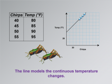
Math Clip Art--Applications of Linear Functions: Cricket Chirps 06 | Math Clip Art--Applications of Linear Functions: Cricket Chirps 06TopicLinear Functions DescriptionThis image builds upon the previous one in the series on applications of linear functions. It shows the same data points as before, but now connected by a straight line. This line represents the continuous relationship between cricket chirps and temperature. |
Graphs of Linear Functions and Slope-Intercept Form |
|
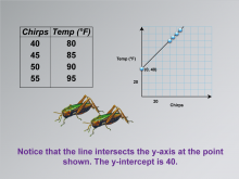
Math Clip Art--Applications of Linear Functions: Cricket Chirps 07 | Math Clip Art--Applications of Linear Functions: Cricket Chirps 07TopicLinear Functions DescriptionThis image in the series on applications of linear functions highlights a crucial feature of the graph: the y-intercept. It shows where the line intersects the y-axis, indicating the y-intercept value. |
Graphs of Linear Functions and Slope-Intercept Form |
|
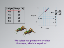
Math Clip Art--Applications of Linear Functions: Cricket Chirps 08 | Math Clip Art--Applications of Linear Functions: Cricket Chirps 08TopicLinear Functions DescriptionThis image in the series on applications of linear functions focuses on calculating the slope of the line. It highlights two specific points on the graph and shows the slope formula used to determine the slope value. |
Graphs of Linear Functions and Slope-Intercept Form |
|
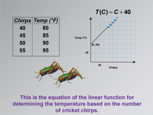
Math Clip Art--Applications of Linear Functions: Cricket Chirps 09 | Math Clip Art--Applications of Linear Functions: Cricket Chirps 09TopicLinear Functions DescriptionThis image in the series on applications of linear functions presents the equation of the linear function. This equation represents the relationship between temperature (T) and the number of cricket chirps (C). |
Graphs of Linear Functions and Slope-Intercept Form |
|
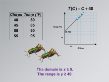
Math Clip Art--Applications of Linear Functions: Cricket Chirps 10 | Math Clip Art--Applications of Linear Functions: Cricket Chirps 10TopicLinear Functions DescriptionThis image concludes the series on applications of linear functions, focusing on the domain and range of the cricket chirps-temperature model. It visually represents the statement "The domain is x ≥ 0. The range is y ≥ 40," which provides crucial information about the limitations and applicability of the linear function. |
Graphs of Linear Functions and Slope-Intercept Form |

|
Math Clip Art--Applications of Linear Functions: Distance vs. Time 01 | Math Clip Art--Applications of Linear Functions: Distance vs. Time 01TopicLinear Functions DescriptionThis image serves as the title card for a series of math clip art illustrations demonstrating applications of linear functions, specifically focusing on distance versus time scenarios. The series, comprising ten images, is designed to explore linear models for speed calculations using distance-time data. This introductory image sets the stage for students to delve into the practical applications of linear functions in real-world contexts. |
Graphs of Linear Functions and Slope-Intercept Form |
|
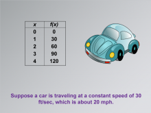
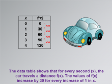
Math Clip Art--Applications of Linear Functions: Distance vs. Time 02 | Math Clip Art--Applications of Linear Functions: Distance vs. Time 02TopicLinear Functions DescriptionThis math clip art image is part of a series illustrating applications of linear functions, focusing on building a linear function model for distance versus time. The image presents a car and a data table, introducing a scenario where a car travels at a constant speed of 30 feet per second, which is approximately 20 miles per hour. This visual representation helps students connect abstract mathematical concepts to real-world situations. |
Graphs of Linear Functions and Slope-Intercept Form |
|
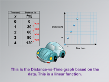
Math Clip Art--Applications of Linear Functions: Distance vs. Time 03 | Math Clip Art--Applications of Linear Functions: Distance vs. Time 03TopicLinear Functions DescriptionThis math clip art image continues the series on applications of linear functions, focusing on the relationship between distance and time. It builds upon the previous image, showing an expanded data table that illustrates how the distance traveled (represented by f(x)) increases for each second (x) that passes. The image emphasizes that for every increase of 1 in x, the values of f(x) increase by 30, corresponding to the car's speed of 30 feet per second. |
Graphs of Linear Functions and Slope-Intercept Form |
|
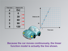
Math Clip Art--Applications of Linear Functions: Distance vs. Time 04 | Math Clip Art--Applications of Linear Functions: Distance vs. Time 04TopicLinear Functions DescriptionThis math clip art image is part of a series demonstrating applications of linear functions, specifically in modeling the relationship between distance and time. The image introduces a graph that visually represents the data from the previous illustrations. It shows a distance-vs-time graph based on the car's movement, clearly depicting a linear function. |
Graphs of Linear Functions and Slope-Intercept Form |
|
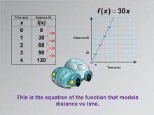
Math Clip Art--Applications of Linear Functions: Distance vs. Time 05 | Math Clip Art--Applications of Linear Functions: Distance vs. Time 05TopicLinear Functions DescriptionThis math clip art image continues the series on applications of linear functions, focusing on the distance-time relationship. It builds upon the previous graph by connecting the data points with a continuous line. The image emphasizes that because the car moves continuously, the linear function model is represented by this unbroken line, not just discrete points. |
Graphs of Linear Functions and Slope-Intercept Form |
|
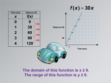
Math Clip Art--Applications of Linear Functions: Distance vs. Time 06 | Math Clip Art--Applications of Linear Functions: Distance vs. Time 06TopicLinear Functions DescriptionThis math clip art image is part of a series illustrating applications of linear functions, specifically modeling the relationship between distance and time. The image introduces the equation f(x) = 30x, which represents the function that models the car's movement. This equation encapsulates the linear relationship between time (x) and distance (f(x)) that has been explored in previous images. |
Graphs of Linear Functions and Slope-Intercept Form |
|
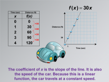
Math Clip Art--Applications of Linear Functions: Distance vs. Time 07 | Math Clip Art--Applications of Linear Functions: Distance vs. Time 07TopicLinear Functions DescriptionThis math clip art image continues the series on applications of linear functions, focusing on the domain and range of the distance-time function. The image emphasizes that the domain of this function is x ≥ 0, and the range is y ≥ 0. This representation helps students understand the practical constraints on the variables in real-world applications of linear functions. |
Graphs of Linear Functions and Slope-Intercept Form |
|
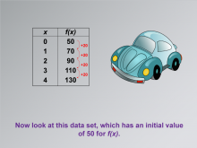
Math Clip Art--Applications of Linear Functions: Distance vs. Time 08 | Math Clip Art--Applications of Linear Functions: Distance vs. Time 08TopicLinear Functions DescriptionThis math clip art image continues the series on applications of linear functions, focusing on the relationship between distance and time. It builds upon previous illustrations by emphasizing that the coefficient of x in the equation f(x) = 30x represents both the slope of the line and the speed of the car. This image reinforces the concept that in a linear function, the rate of change remains constant throughout. |
Graphs of Linear Functions and Slope-Intercept Form |
|
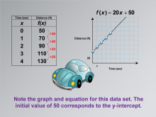
Math Clip Art--Applications of Linear Functions: Distance vs. Time 09 | Math Clip Art--Applications of Linear Functions: Distance vs. Time 09TopicLinear Functions DescriptionThis math clip art image is part of a series illustrating applications of linear functions, with a focus on the distance-time relationship. It presents a new scenario with a car and an updated data table. The image likely introduces a different speed or starting point, allowing students to compare and contrast with the previous example and explore how changes in initial conditions affect the linear function. |
Graphs of Linear Functions and Slope-Intercept Form |
|
Math Clip Art--Applications of Linear Functions: Distance vs. Time 10 | Math Clip Art--Applications of Linear Functions: Distance vs. Time 10TopicLinear Functions DescriptionThis math clip art image concludes the series on applications of linear functions in the context of distance versus time relationships. It presents a linear graph corresponding to the data table introduced in the previous image. This visual representation allows students to see how the new scenario translates into a graphical form, reinforcing the connection between tabular data and its linear graph. |
Graphs of Linear Functions and Slope-Intercept Form |

|
Math Clip Art--Applications of Linear Functions: Hooke's Law 01 | Math Clip Art--Applications of Linear Functions: Hooke's Law 01TopicLinear Functions DescriptionThis image serves as the title card for a series of illustrations demonstrating applications of linear functions, specifically focusing on Hooke's Law. The series, comprising eight images, explores the relationship between force and displacement in springs, showcasing how linear models can represent real-world phenomena. |
Graphs of Linear Functions, Slope-Intercept Form and Proportions |
|
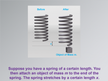
Math Clip Art--Applications of Linear Functions: Hooke's Law 02 | Math Clip Art--Applications of Linear Functions: Hooke's Law 02TopicLinear Functions DescriptionThis image is part of a series illustrating applications of linear functions, focusing on Hooke's Law. It depicts a spring before and after being stretched by a weight, visually representing the fundamental concept of Hooke's Law. The illustration shows a spring in its original state and then stretched by an object of mass m, extending by a length x. This visual representation helps students understand the relationship between the applied force (weight) and the resulting displacement of the spring, which forms the basis of the linear function in Hooke's Law. |
Graphs of Linear Functions, Slope-Intercept Form and Proportions |

|
Math Clip Art--Applications of Linear Functions: Hooke's Law 02 | Math Clip Art--Applications of Linear Functions: Hooke's Law 02TopicLinear Functions DescriptionThis image is part of a series illustrating applications of linear functions, focusing on Hooke's Law. It depicts a spring before and after being stretched by a weight, visually representing the fundamental concept of Hooke's Law. The illustration shows a spring in its original state and then stretched by an object of mass m, extending by a length x. This visual representation helps students understand the relationship between the applied force (weight) and the resulting displacement of the spring, which forms the basis of the linear function in Hooke's Law. |
Graphs of Linear Functions, Slope-Intercept Form and Proportions |
|
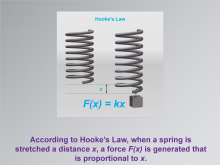
Math Clip Art--Applications of Linear Functions: Hooke's Law 03 | Math Clip Art--Applications of Linear Functions: Hooke's Law 03TopicLinear Functions DescriptionThis image is a continuation of the series on applications of linear functions, specifically illustrating Hooke's Law. It builds upon the previous image by introducing the mathematical equation F(x) = kx, which is the core of Hooke's Law. The illustration shows that when a spring is stretched a distance x, a force F(x) is generated that is proportional to x. This visual representation, combined with the equation, helps students understand the linear relationship between force and displacement in springs. |
Graphs of Linear Functions, Slope-Intercept Form and Proportions |

|
Math Clip Art--Applications of Linear Functions: Hooke's Law 03 | Math Clip Art--Applications of Linear Functions: Hooke's Law 03TopicLinear Functions DescriptionThis image is a continuation of the series on applications of linear functions, specifically illustrating Hooke's Law. It builds upon the previous image by introducing the mathematical equation F(x) = kx, which is the core of Hooke's Law. The illustration shows that when a spring is stretched a distance x, a force F(x) is generated that is proportional to x. This visual representation, combined with the equation, helps students understand the linear relationship between force and displacement in springs. |
Graphs of Linear Functions, Slope-Intercept Form and Proportions |
|
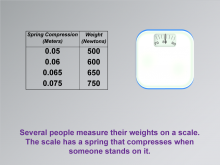
Math Clip Art--Applications of Linear Functions: Hooke's Law 04 | Math Clip Art--Applications of Linear Functions: Hooke's Law 04TopicLinear Functions DescriptionThis image is part of a series demonstrating applications of linear functions, focusing on Hooke's Law. It presents a practical application of the law by showing a data table alongside a weight scale, illustrating how Hooke's Law applies to everyday objects. |
Graphs of Linear Functions, Slope-Intercept Form and Proportions |

|
Math Clip Art--Applications of Linear Functions: Hooke's Law 04 | Math Clip Art--Applications of Linear Functions: Hooke's Law 04TopicLinear Functions DescriptionThis image is part of a series demonstrating applications of linear functions, focusing on Hooke's Law. It presents a practical application of the law by showing a data table alongside a weight scale, illustrating how Hooke's Law applies to everyday objects. |
Graphs of Linear Functions, Slope-Intercept Form and Proportions |
|
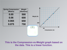
Math Clip Art--Applications of Linear Functions: Hooke's Law 05 | Math Clip Art--Applications of Linear Functions: Hooke's Law 05TopicLinear Functions DescriptionThis image is a continuation of the series on applications of linear functions, specifically illustrating Hooke's Law. It builds upon the previous image by presenting a graph of the data collected from the weight scale experiment. The illustration shows a Compression-vs-Weight graph based on the data from the weight scale. The graph displays a clear linear relationship, with data points connected by a straight line. This visual representation helps students see how the abstract concept of a linear function manifests in real-world data. |
Graphs of Linear Functions, Slope-Intercept Form and Proportions |
|
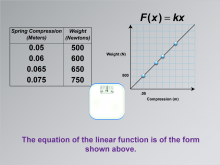
Math Clip Art--Applications of Linear Functions: Hooke's Law 06 | Math Clip Art--Applications of Linear Functions: Hooke's Law 06TopicLinear Functions DescriptionThis image is part of a series demonstrating applications of linear functions, specifically focusing on Hooke's Law. It builds upon the previous images by introducing the general form of the linear function equation that describes the relationship observed in the weight scale experiment. |
Graphs of Linear Functions, Slope-Intercept Form and Proportions |

|
Math Clip Art--Applications of Linear Functions: Hooke's Law 06 | Math Clip Art--Applications of Linear Functions: Hooke's Law 06TopicLinear Functions DescriptionThis image is part of a series demonstrating applications of linear functions, specifically focusing on Hooke's Law. It builds upon the previous images by introducing the general form of the linear function equation that describes the relationship observed in the weight scale experiment. |
Graphs of Linear Functions, Slope-Intercept Form and Proportions |